Introduction to using LSDTopoTools

Return to main LSDTopoTools landing page

1. Introduction and overview

This document takes you through an inital LSDTopoTools analysis. Through the tutorials contained here we will demonstrate how our analysis programs run: they all share a common interface.

Before you start

Before you start you need to install LSDTopoTools. If you haven’t done that, please follow the link below.

Instructions on how to install LSDTopoTools

In addition, you will need to use some basic linux shell commands. If you have never done this before I suggest reading this brief introduction: Basic use of the linux shell.

1.1. The basic structure of an analysis

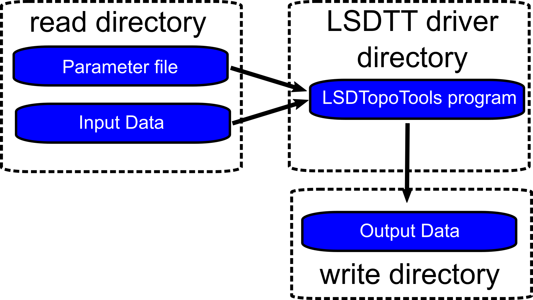
Our analyses are packaged into separate programs. They are run from the Linux shell. If you don’t have Linux, don’t worry, we use containers to create a Linux environment in your computer (see installation instructions). All of our programs operate the same way:

You call the programs (such as lsdtt-basic-metrics and lsdtt-channel-extraction) from the command line.
These programs work on topographic data, and they use a parameter file that tells the programs what to do with the data.

The basic structure looks like this:

The basic structre of an LSDTopoTools analysis

Figure 1. All LSDTopoTools analyses work like this.

1.1.1. Running a typical analysis for lsdtt-basic-metrics

In the next section we will walk you though an analysis. However, reading this will help you understand where you are going, so we recommend you read the whole thing!

You run the program from a terminal window
You can supply the program with:
- a directory name
- a parameter file name
- both of these things
- none of these things
If you don’t supply a parameter filename, the program will assume the parameter file is called LSDTT_parameters.driver

If the parameter file doesn’t exist, you will get an error message.

Any of the following calls to one of the programs will work, as long as your files are in the right place:

$ lsdtt-basic-metrics
$ lsdtt-basic-metrics /LSDTopoTools/data/A_project
$ lsdtt-basic-metrics AParameterFile.param
$ lsdtt-basic-metrics /LSDTopoTools/data/A_project AParameterFile.param

The program name (lsdtt-basic-metrics), the directory name (/LSDTopoTools/data/A_project) and the parameter file name (AParameterFile.param) will change but all LSDTopoTools calls follow this same basic structure.

Now, all parameter files have these basic elements in them:

read path: /LSDTopoTools/data/A_project
write path: /LSDTopoTools/data/A_project
read fname: Data_prefix
write fname: Data_prefix

You need to change the path and fnames to reflect your data!
If the read path and write path are not specified, then the program will assume the data is in the same directory as the program is being run.

1.1.2. How do I change my parameter files?

You can edit your parameter files in a text editor: this is just a program that edits plain text. DO NOT use a word processor. These modify file types.

There are many options for text editors but we like: * Brackets works on any operating system. * Atom also works on any operating system.

If you are on Windows then pspad is also quite good.

A note on read and write paths

If you leave read path and write path blank, LSDTopoTools programs will assume the data is in the current directory. You can find out what the current directory is by typing pwd at the command prompt. As long as your data is in the same directory as your parameter file you won’t need to bother with this section at all. 99% of LSDTopoTools users can skip this section.

Editing read and write paths can be a bit annoying if you are moving data from place to place, so we have a python script, called LSDTTParamfileUpdater.py that updates the paths in the parameter file for you. The way you run that is:

Download the script into your data folder (i.e. in the second terminal window you have open above):

$ wget https://raw.githubusercontent.com/LSDtopotools/LSDAutomation/master/LSDTTParamfileUpdater.py

Run the file
```
$ python LSDTTParamfileUpdater.py
```
Again, you don’t need to do any of this if your data is in the same directory as your parameter file and you have left the read path and write path out of your parameter file.

2. Basic analyses in LSDTopoTools using the lsdtt-basic-metrics program

This chapter will walk you through some basic topographic analysis using our program lsdtt-basic-metrics. This program can extract topographic metrics like slope, aspect and curvature. Alongside these metrics it can also extract channel networks, and get drainage areas. The program is intended for everyday data processing. A number of these operations are available in GIS software, but we tend to prefer LSDTopoTools because:

The slope and curvature metrics in typical GIS software only uses information from the nearest pixels. We fit a polynomial surface from a neighbourhood of pixels. See Hurst et al., 2012, DOI: 10.1029/2011JF002057 and Grieve et al., 2016, doi:10.5194/esurf-4-627-2016 for the rationale.
Our channel extractions for the d8 method are based on the FASTSCAPE algorithm and are MUCH faster than running channel extraction in typical GIS software.
The program does some data preprocessing behind the scenes that you would need to do manually in a GIS. For example, if the nodata values are messed up, LSDTopoTools can fix these.
We have automated some basin selection routines, which again you would need to do by hand in a GIS.
Our channel extraction spits out networks with drainage areas, locations, chi coordinates and all sorts of other goodies that would take ages on a GIS.

The examples in this section are used for both LSDTopoTools workshops as well as in the University of Edinburgh course, Eroding Landscapes.

2.1. Your first analysis using LSDTopoTools

We are going to run an LSDTopoTools2 program that is used for basic topographic analysis. If you have installed the programs already you just need to make sure that they are in your path. See the installation instructions.

Before you start

Before you start you need to install LSDTopoTools. If you haven’t done that, please follow the link below.

Instructions on how to install LSDTopoTools

In addition, you will need to use some basic linux shell commands. If you have never done this before I suggest reading this brief introduction: Basic use of the linux shell.

2.1.1. Get the test data

If you have followed the installation instructions and grabbed the example data, you already have what you need! If not, follow the steps below:

If you are using a docker container, just run the script:
```
# Get_LSDTT_example_data.sh
```
If you are on a native linux or using the University of Edinburgh servers, do the following:
1. If you have installed LSDTopoTools, you will have a directory somewhere called LSDTopoTools. Go into it.
2. Run the following commands (you only need to do this once):
  $ mkdir data $ cd data $ wget https://github.com/LSDtopotools/ExampleTopoDatasets/archive/master.zip $ unzip master.zip $ mv ./ExampleTopoDatasets-master ./ExampleTopoDatasets $ rm master.zip
3. WARNING: This downloads a bit over 150Mb of data so make sure you have room.

2.1.2. Run an analysis

Go into the directory with this data: cd ExampleTopoDatasets/BasicMetricsData.
If you have installed LSDTopoTools correctly, you should just be able to call lsdtt-basic-metrics:
```
$ lsdtt-basic-metrics WA_BasicMetrics01.driver
```
This will spit out some information to you screen. It will also make a hillshade of the DEM, which is called WA_FirstExample_hs.bil.

2.1.3. Look at the data

You can look at this raster in QGIS. We have some instructions for QGIS, if you want to see instructions for adding data click here.
Open QGIS and load the raster. The new raster is in the same directory with your other data and is called WA_FirstExample_hs.bil.The data will look like this: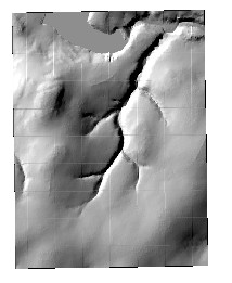

Figure 2. A hillshade of the Whiteadder catchement
As you can see, the DEM has quite a few artefacts. There isn’t much we can do about that, I’m afraid.

2.2. Getting surface metrics

Now we will get a bit more information about the DEM. Again, we will run an LSDTopoTools program (lsdtt-basic-metrics) that will ingest a raster WA.bil and spit out some new rasters.

Start by running the program with the second driver file:
```
$ lsdtt-basic-metrics WA_BasicMetrics02.driver
```

This does more stuff. We can look at the driver file:

# Parameters for extracting simple surface metrics
# Comments are preceded by the hash symbol

# These are parameters for the file i/o
read fname: WA
write fname: WA_SecondExample
channel heads fname: NULL

# Parameters for surface metrics
surface_fitting_radius: 11
print_slope: true
print_aspect: true
print_curvature: true
print_tangential_curvature: true

In this case the program is printing slope, aspect, curvature, and tangential curvature rasters. They have filenames that reflect their contents so have a look. Slope tells you how steep the landscape is, aspect which direction the surface is pointing, curvature how, uh, curvy the landscape is (mathematically it is how quickly slope changes in space) and the tangential curvature is how curvy the landscape is in the direction of steepest descent. Essentially tangential curvature tells you how tightly curved contours are and is useful for finding valleys.
The way these are calculated is by fitting a surface of radius surface_fitting_radius to the points in the DEM and then calculating derivatives of that surface.

2.2.1. Questions and tasks for surface metrics

Try changing the surface_fitting_radius. What happens?

2.3. Drainage area and channel extraction

Finally, we will compute some drainage areas and extract a channel network. To do this run the driver file WA_BasicMetrics03.driver.

Run the program using:

$ lsdtt-basic-metrics WA_BasicMetrics03.driver

Yet more stuff will come out. Some are drainage area rasters, but there is also a csv file, WA_ThirdExample_CN.csv.
You will get a file with points, which you can load into QGIS. You can read about how to do that in our QGIS instructions. You will get something that looks a bit like this:

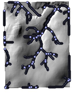Figure 3. A simple channel network

2.3.1. Questions for channel extraction.

Try changing the threshold_contributing_pixels parameter. What happens to the channel network?
More advanced: You can get a smoothed elevation raster with the following driver file line: print_smoothed_elevation: true. Try creating a smoothed elevation raster and then using this smoothed raster for the drainage extraction. You will need to change the read fname parameter to reflect the smoothed raster.

2.4. Summary

You now have seen the basic interface of LSDTopoTools programs, got a small taste of Linux, and know a few things about QGIS. From here you should be able to move on to more advanced topographic analysis.

3. More advanced options in lsdtt-basic-metrics

One of the most common operations when analysing topographic data is extracting channel networks. We have an entire package for that, which has a number of different channel extraction algorithms.

However, many users just want channels extracted with the minimum of fuss and so we provide a simple channel profile extraction tool in lsdtt-basic-metrics.

3.1. What channels do you want? Selecting basins

Sometimes you don’t want every channel in the landscape, but only particular channels. We have some basin selection tools for this.

The next driver file has some options for selecting basins (WA_BasicMetrics04.driver):

# These are parameters for the file i/o
read fname: WA
write fname: WA_FourthExample
channel heads fname: NULL

# Basic channel network
threshold_contributing_pixels: 5000
print_junctions_to_csv: true

# Convert to json
convert_csv_to_geojson: true

# Getting the basins
find_basins: true
minimum_basin_size_pixels: 10000
maximum_basin_size_pixels: 100000000
only_take_largest_basin: false

# Print the basin raster
print_basin_raster: true

The key elements here are:

find_basins: true This tells the program to find specific basins
minimum_basin_size_pixels: 10000 This tells the program to get basins at least this big. They must be smaller than maximum_basin_size_pixels.
only_take_largest_basin When false it finds all basins in the size window, whereas if tru you only get the larges basin.
print_basin_raster: true this prints a basin raster.

Run the driver and have a look at the new files.

If you load the basin raster in QGIS (it has the extension AllBasins)

Figure 4. Basins extracted from the DEM

You can try modifying some of the parameters like the minimum and maximum basin size and the flag only_take_largest_basin to see what you get.

3.1.1. Geojson data

If you use the switch convert_csv_to_geojson: true the csv files will be converted to geojson files which can be loaded directly as shapefiles in a GIS. Have a look at our QGIS documents; we have instructions for loading "vector" data. Geojson files contain GIS-readable vector data.

3.2. Picking basins

If you ran the previous driver you will get a geojson file that has _JN.geojson in the name. If you load this data in a GIS you will see something like this: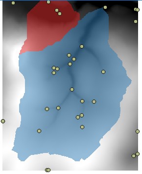

Figure 5. Junctions in the DEM

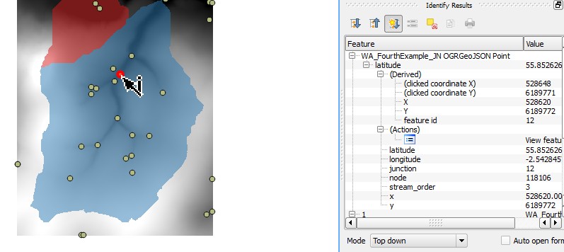Figure 6. Junction information in the DEM

You can see in the table to the right the junction number is 12.
If you want to pick certain junctions you can make a text file and just write the junction numbers you want in that text file.
We have added a junctions file in the directory with the data called selected_WA.junctions. It has a few junctions picked. The line to add to the parameter file are:
```
BaselevelJunctions_file: /LSDTopoTools/dataExampleTopoDatasets/selected_WA.junctions
```
This line needs the entire path to your file. So you will probably need to go into the file and change the filename to match your directory structure.
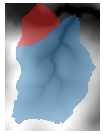
Run the next parameter file (WA_BasicMetrics05.driver) and have a look at the basins generated. They will look something like this:

Figure 7. Selected basins

3.3. An important note on basin selection.

In LSDTopoTools basins are selected on the basis of junctions. But junctions have two or more contributing channels! The basin selected by a junction includes the channel going downstream that stops one pixel before the next junction. In this way we can select basins that are representative of a given Strahler order.

3.4. Getting a channel network with more information

The next driver file is WA_BasicMetrics06.driver and it looks like this:

# These are parameters for the file i/o
read fname: WA
write fname: WA_SixthExample
channel heads fname: NULL

# Basic channel network
threshold_contributing_pixels: 5000

# Convert to json
convert_csv_to_geojson: true

# Getting the basins
find_basins: true
maximum_basin_size_pixels: 100000000
only_take_largest_basin: true

# Print the basin raster
print_chi_data_maps: true

The key element of this file is print_chi_data_maps: true. This prints a channel network that you can load into a GIS (the file has the extension _chi_data_map):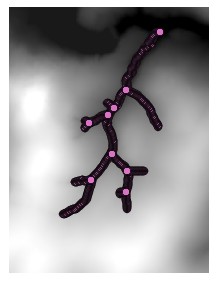

Figure 8. The channel network produced from the chi data maps
This looks a bit like the old channel network but the file contains much more information. If you open the csv file you will see the location of the points but also drainage area, elevation, flow distance, keys for identifying tributaries, and something called the chi coordinate, which you can read all about in a different part of the documentation.
You could, for example, make a chi-elevation plot using the data in the csv file:

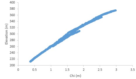Figure 9. A chi-elevation plot for the basin

Appendix A: Analysis options for the lsdtt-basic-metrics program

All LSDTopoTools parameter files have the same format:

# comment
keyword: value
keywords with spaces: value

The parameter file has a specific format, but the filename can be anything you want. We tend to use the extensions .param and .driver for these files, but you could use the extension .MyDogSpot if that tickled your fancy.

LSDTopoTools parameter file format

The # denotes a comment. The program will ignore line that start with this symbol.
Keywords or phrases are followed by a colon (:).
Keywords MUST be spelled exactly. They are not case sensitive. If you have a leading space it will not work. If you have a space before the colon (:) it will not work.
The order of the keywords do not matter.
If a keyword is not found, a default value is assigned. That is, you don’t need to worry about forgetting an essential parameter since they all are assigned default values.

Input format

Below are options for the parameter files. For these programs there are options for converting to point data, which requires georeferencing. Therefore, all DEMs must be in ENVI bil format (DO NOT use ArcMap’s bil format: these are two different things. See the section [Preparing your data] if you want more details). The reason we use bil format is because it retains georeferencing which is essential to our file output since many of the files output to csv format with latitude and longitude as coordinates.

A.1. Basic file input and output

Table 1. File input and output options. **These do not have defaults and MUST be declared**.
Keyword	Input type	Description
write path	string	The path to which data is written. The code will NOT create a path: you need to make the write path before you start running the program.
read path	string	The path from which data is read.
write fname	string	The prefix of rasters to be written without extension. For example if this is `Test` and you have selected `bil` format then a fill operation will result in a file called `Test_Fill.bil`.
read fname	string	The filename of the raster to be read without extension. For example if the raster is `MyRaster.bil`, read fname will be `MyRaster`.
channel heads fname	string	The filename of a channel heads file. You can import channel heads. If this is set to `NULL` then the channels will be calculated using a pixel threshold.

A.2. DEM preprocessing

Table 2. DEM preprocessing. These just help you clean data and perform very basic operations.
Keyword	Input type	Default value	Description
minimum_elevation	float	0	If you have the `remove_seas` keyword set to true, the program will change any elevation node below this value to NoData.
maximum_elevation	float	30000	If you have the `remove_seas` keyword set to true, the program will change any elevation node above this value to NoData.
remove_seas	bool	false	If true, this changes extreme value in the elevation to NoData.
min_slope_for_fill	float	0.001	The minimum slope between pixels for use in the fill function.
raster_is_filled	bool	false	If true, the code assumes the raster is already filled and doesn’t perform the filling routine. This should save some time in computation, but make sure the raster really is filled or else you will get segmentation faults!
carve_before_fill	bool	false	If true, this runs a carving algoriothm before the fill function (Algorithm from Lindsay 2016). This breaches dams so that you don’t get giant flat areas.
only_check_parameters	bool	false	If true, this checks parameter values but doesn’t run any analyses. Mainly used to see if raster files exist.

A.3. Raster trimming options (more preprocessing)

Table 3. These are more preprocessing routines specifically for trimming rasters
Keyword	Input type	Default value	Description
remove_nodes_influenced_by_edge	bool	false	If true, this removes all pixels that are influenced by the edge or nodata. Influence is determined by D8 flow: The code starts at any node adjacent to the edge or nodata and then "erases" (converts to no data) all pixels downstream of this subset of pixels.
isolate_pixels_draining_to_fixed_channel	bool	false	If true, this only retains pixels from the DEM that drain to a set of points (usually a channel), which is stored in the fixed channel csv (see below).
fixed_channel_csv_name	string	single_channel_nodes	This is the name of a csv file that contains a list of nodes. It looks for node indices (it can find "ni", "nodeindex", or "index" in the csv) so is actually rather crap since you will need to update this file any time you change the raster. SMM needs to change this to read lat-long so it is not DEM-specific
print_trimmed_raster	bool	false	This is a slightly different trimmer: it finds the largest rectangular raster without nodata around the edges and prints to file.
trimming_buffer_pixels	int	0	THis is a parameter for the `print_trimmed_raster` option: it creates a buffer between the last nodata node and the edge of the DEM.

A.4. Basic data output

Table 4. Basic printing operations. For simple rasters and network data that doesn’t require chi analysis.
Keyword	Input type	Default value	Description
convert_csv_to_geojson	bool	false	If true, this converts any csv file (except for slope-area data) to geojson format. This format takes up much more space than csv (file sizes can be 10x larger) but is georeferenced and can be loaded directly into a GIS. Also useful for webmapping. It assumes your raster is in UTM coordinates, and prints points with latitude and longitude in WGS84.
print_raster_without_seas	bool	false	If true, prints a raster that has removed the seas (and very high peaks). This is useful if your NoDataValue is not registering and you use the `minimum_elevation`, `maximum_eleation`, and `remove_seas` flags to correct this. WARNING! This overwrites your original raster.
print_fill_raster	bool	false	If true, prints the fill raster.
write_hillshade	bool	false	If true, prints the hillshade raster. The format of this is stupidly different from other printing calls for a stupid inheritance reason. Try to ignore. Most GIS routines have a hillshading options but for some reason they look crappier than our in-house hillshading. I’m not sure why but if you want a hillshade I recommend using this function.
print_distance_from_outlet	bool	false	Prints a raster that gives the distance from the outlet.
print_wiener_filtered_raster	bool	false	This returns a filtered raster using something called a Wiener filter. It is a rather fancy way to smooth topography. Note that this uses a memory-hungry fourier transform and so will struggle or even crash on large DEMs.

A.5. Surface fitting

Table 5. These are options for polynomial surface fitting.
Keyword	Input type	Default value	Description
surface_fitting_radius	float	30	The radius of the polynomial window over which the surface is fitted. If you have lidar data, we have found that a radius of 5-8 metres works best.
print_smoothed_elevation	bool	false	Prints a raster of elevations that have been smoothed over the polynomial window
print_slope	bool	false	If true, prints the topographic gradient raster.
print_aspect	bool	false	If true, prints the aspect raster.
print_curvature	bool	false	If true, prints the curvature raster.
print_planform_curvature	bool	false	If true, prints the planform curvature raster. That is the curvature of the countour lines.
print_profile_curvature	bool	false	If true, prints the profile curvature raster. That is the curvature along the line of steepest descent.
print_tangential_curvature	bool	false	If true, prints the tangential curvature raster. This is the curvature perpendicular to the line of steepest descent. A bit like the planform curvature but adjusted for slope.
print_point_classification	bool	false	If true, prints a point classification raster. This takes the value 1 if there is a peak, 2 if there is a depression and 3 if there is a saddle.
print_directional_gradients	bool	false	If true, prints two rasters, for sloipes in each of the cardinal directions
calculate_basin_statistics	bool	false	If true, it goes thrugh the basin selection, and then prints statistics about slope and/or curvature for that basin. You must have print_slope and/or print_curvature set to true for this to work. The output goes into a csv file.
calculate_window_size	bool	false	It this is set to true, runs a calculation to estimate the best window size for surface fitting. Warning: this is computationally expensive and might take a while.

A.6. Roughness calculation

Table 6. These are options for calculationg landscape roughness
Keyword	Input type	Default value	Description
REI_critical_slope	float	1.0	Critical slope for the rock exposure index calculation
REI_window_radius	float	10.0	Radius for the window for the rock exposure index calculation
print_REI_raster	bool	false	If true, prints the REI to a raster
print_roughness_rasters	bool	false	If true, prints the S1,S2, and S3 rasters. See Milodwski et al, ESURF for details.
roughness_radius	float	3.0	Radius for the window for the roughness calculation

A.7. Drainage area extraction

Table 7. These are options for drainage area extraction.
Keyword	Input type	Default value	Description
surface_fitting_radius	float	30	The radius of the polynomial window over which the surface is fitted. If you have lidar data, we have found that a radius of 5-8 metres works best.
print_dinf_drainage_area_raster	bool	false	If true, prints drainage area calculated using the d-infinity algorithm.
print_d8_drainage_area_raster	bool	false	If true, prints drainage area calculated using the d8 algorithm. This is simply the steepest of the 8 nearest neighbours.
print_QuinnMD_drainage_area_raster	bool	false	If true, prints drainage area calculated using the Quinn algorithm. This is a multiple flow direction algorithm.
print_FreemanMD_drainage_area_raster	bool	false	If true, prints drainage area calculated using the Freeman algorithm. This is a multiple flow direction algorithm.
print_MD_drainage_area_raster	bool	false	If true, prints drainage area calculated using the multidirectional algorithm. This is a multiple flow direction algorithm. Unlike the Quinn and Freeman algorithms it makes no attempt whatsoever to control dispersion.

A.8. Basic channel extraction and printing

This simply gets a channel network and prints its location. It is a rather rudimentary way of seeing where channels are. More advanced options are in the next table.

Table 8. These are options for drainage area extraction.
Keyword	Input type	Default value	Description
print_stream_order_raster	bool	false	If true, prints the stream order raster (but printing this to csv is more efficient, use `print_channels_to_csv`).
print_channels_to_csv	bool	false	Prints the channel network to a csv file. Includes stream order and other useful information. Much more memory efficient than printing the whole raster. It prints all channel nodes across the DEM rather than printing nodes upstream of selected basins. If you want to see the channels selected for chi analysis use `print_chi_data_maps`.
print_junction_index_raster	bool	false	If true, prints the junction index raster (but printing this to csv is more efficient, use `print_junctions_to_csv`).
print_junctions_to_csv	bool	false	Prints the junction indices to a csv file. Much more memory efficient than printing the whole raster.
print_junctions_angles_to_csv	bool	false	Prints the junction angles of each junction to a csv file. This has rather a lot of data outputs. It rejects junctions with more than two donors. It records the order of the junction and each of the two donors. It also records the drainage area of the junction and the two donors. It records the bearing of each of the three channels (all pointing away from the junction, so the two donors point upstream and the channel below the junction points downstream). It also records the angle between the two donors as well as the angle between the D1 and the downstream channel, and D2 and the downstream channel.
extract_single_channel	bool	false	If true, this takes a single source (entered as a lat-long in a csv file, see below) and follows it doenstream. A very easy way to get statistics from a single channel. The channel records flow distance and drainage area.
use_dinf_for_single_channel	bool	false	If true, records the dinf drainage area rather than D8 drainage area in the single channel csv
channel_source_fname	string	single_channel_source	Name of a csv file that has latitude and longitude as column headers. Only takes the first item in the file as the channel source. Used by `extract_single_channel`.

A.9. More advanced channel and basin selection

These options give you a bit of control over selecting basins.

If you just want the largest complete basin, set find_largest_complete_basins: true AND maximum_basin_size_pixels: 10000000000000 (or any really big number).

Table 9. Options for determining which channels and basins to analyse, including settings for the fill function.
Keyword	Input type	Default value	Description
find_basins	bool	false	If this is true, it i) Gets all the basins in a DEM and takes those between the `minimum_basin_size_pixels` and `maximum_basin_size_pixels`. It then removes basins that are influenced by the edge of the DEM, and then removes nested basins. The reason for removing basins draining the edge is that all drainage areas and chi coordinates require that the basin is complete. If not, your areas and chi coordinate, will be incorrect.
BaselevelJunctions_file	string	NULL	You can write a file that contains a list of junction numbers (to see where they are, use `print_junctions_to_csv`) to get basins above specific junctions only. The file format is just a list of integers.
CHeads_file	string	NULL	This reads a channel heads file. It will supercede the `threshold_contributing_pixels` flag. That is, if you give a valid CHeads filename the code will ignore the threshold pixels and use the sources in the file instead. You can calculate channel heads using our channel extraction tools. The file needs to be a csv file and you pass the filename WITHOUT EXTENSION. The format of the filename is one with 5 columns: `node_index,row,col,x,y`. The `x,y` coordinates are in local UTM coordinates.
threshold_contributing_pixels	int	1000	The number of pixels required to generate a channel (i.e., the source threshold).
minimum_basin_size_pixels	int	5000	The minimum number of pixels in a basin for it to be retained. This operation works on the baselevel basins: subbasins within a large basin are retained.
maximum_basin_size_pixels	int	500000	The maximum number of pixels in a basin for it to be retained. This is only used by `find_complete_basins_in_window` but that algorithm for selecting basins is the default.
extend_channel_to_node_before_receiver_junction	bool	true	If true, the channel network will extend beyond selected baselevel junctions downstream until it reaches the pixel before the receiver junction. If false, the channel simply extends upstream from the selected basin. The reason for this switch is because if one if extracting basins by drainage order, then the, say, a 2nd order drainage basin starts at the node immediately upstream of the most upstream 3rd order junction.
only_take_largest_basin	bool (true or 1 will work)	false	If this is true, a chi map is created based only upon the largest basin in the raster.
print_basin_raster	bool	false	If true, prints a raster with the basins. IMPORTANT! This should be set to true if you want to use any of our python plotting functions that use basin information. Note that if this is true it will also print csv files with basin numbers and source numbers to assist plotting.
print_chi_data_maps	bool	false	This prints the channel networks (a bit like `print_channels_to_csv`) but contains MUCH more informatioon: elevation, flow distance, dranage area (from d8), the chi coordinate (have a look at our chi documentation for more details) and various keys to sources and basins so you can colour or sort channels by basin or tributary if you want. If you are going to work with channels using LSDTT_BasicMetrics this is the output to use.

A.9.1. Basic parameters for the chi coordinate

Table 10. Parameters for calculating the chi coordinate.
Keyword	Input type	Default value	Description
A_0	float	1	The A₀ parameter (which nondimensionalises area) for chi analysis. This is in m². Note that when A₀ = 1 then the slope in chi space is the same as the channel steepness index (often denoted by k_s).
m_over_n	float	0.5	The m/n parameter (sometimes known as the concavity index) for calculating chi. Note that if you do any m/n analysis (either `calculate_MLE_collinearity` or `print_profiles_fxn_movern_csv`) this m/n value will be replaced.

A.10. Example parameter files

We have a number of example parameter files in the repository LSDTT_chi_examples. The chapter on examples will walk you through the various things these files do.