QGIS Notes and Tips

Preface by Simon Mudd

This is a collection of notes on simple operations within QGIS. It stems from a course at Edinburgh where the topic is Geomorphology but for the course project students need to analyse topographic data. This is not meant to be a course on QGIS! However if you are just looking to get started with the very basics you might find it helpful.

This document is part of a family of documents on topographic analysis using LSDTopoTools; you can migrate back to the main landing page by clicking this link.

1. Background and Motivation

QGIS is a free and open source Geographic Information System (GIS). This book contains instructions on how to perform basic operations within QGIS. It is not meant to be a QGIS course, but rather should get you started if you just want to look at some data.

If you want to actually gain a deeper understanding of QGIS there are many excellent resources:

http://www.qgistutorials.com/en/docs/learning_resources.html A curated collection of QGIS learning resources
http://qgis-tutorials.mangomap.com/ A series of brief videos explaining simple QGIS tasks
http://gis.stackexchange.com/questions/3651/where-to-find-qgis-tutorials-and-web-resources Another list of QGIS resources.

In addition, QGIS now has a large, active and growing user community and if you type in a question about QGIS into a search engine you are almost certain to find a solution to your problem.

So, with all of these fantastic resources, why, you ask, am I writing these notes? In short, my students need to do a very specific subset of GIS tasks; these tasks are explained here. Hopefully the result is more efficient then sending many students separately to the myriad of QGIS websites.

1.1. The QGIS version used for this book

We use the long term release (LTE) version of QGIS 2.14 (Essen): http://www.qgis.org/en/site/forusers/download.html

1.2. Basic QGIS layout

When you load QGIS you will see a bunch of toolbars and panels. This brief section describes a few of the key elements. If you want more detail see the QGIS documentation: https://docs.qgis.org/2.2/en/docs/training_manual/introduction/overview.html

The basic layout of QGIS looks like this:

Figure 1. Basic QGIS 2.14 layout

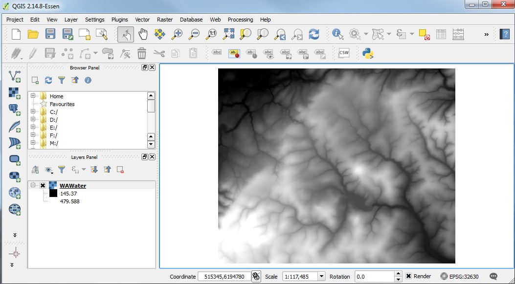
On the right you will see some "panels". You can drag these around the screen if you like. In addition, you can right click in the menu bars near the top of the window to select different panels.

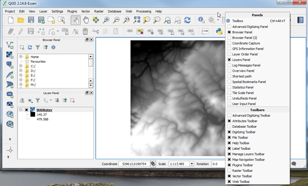
Figure 2. Right click to select panels

If you accidentally remove a panel you can get it back by right clicking near the top of the page and reselecting the panel.

The layers panel shows you what data you currently have loaded into QGIS (see bottom left in above images: there is one layer loaded called WAWater).

In the screen is also a panel for adding data, which is called the Manage layers toolbar:

Figure 3. The layers toolbar

In the above image I have moved the toolbar to display horizontally; any of these toolbars or panels can be moved around by clicking and dragging them.

If you look below the actual data window, which in QGIS is called the map canvas (where in the above images the layer WAWater is displayed), you see some important information in what QGIS calls the status bar.

Figure 4. The status bar

This contains the location of your mouse pointer in the map canvas, some information about scale and rotation of your map, and importantly the projection. Map projections all have something called an EPSG number, so for example the British National Grid is EPSG:27700, the global WGS84 projection is EPSG:4326, and WGS UTM coordinates for the northern hemisphere are EPSG:326XX where the XX is the zone number, and EPSG:327XX is for the southern hemisphere. You can read more on projections in our appendix.

Now that you have some idea about what the main QGIS window looks like, it is time to move on and add some data.

2. Adding data

This chapter details the basics of adding data to QGIS. Before you add any data, you should know that geographic data comes in two basic flavours: raster and vector data.

Raster data is built on a regular grid. It has pixels that contain different values. If the raster data has "bands" it just means that there are multiple values assigned to each pixel. The most common version of raster bands is for image data that has a red, green and blue band (RGB).
Vector data, in a GIS context, actually means a number of related data types that contain locations at specific points. So points, lines or polylines, and polygons are all considered vector data. You can read about the differences here: https://en.wikipedia.org/wiki/GIS_file_formats#Vector_formats

For each of these two data types, there are many different file formats that QGIS can read. If you want to read about them the QGIS documentation has lists for supported vector file formats, and for rasters QGIS supports anything supported by another bit of software called GDAL: here is the list of supported raster formats. In the following sections we will very briefly explain how to import these data into QGIS.

2.1. Adding raster data

To add raster data you need to click on the part of the manage layers toolbar that looks like a checkerboard:

Figure 5. Adding raster data

In newer versions of QGIS the add data button looks like this:

Figure 6. Adding data in QGIS 3+

There are enormous numbers of raster file formats. These can broadly be broken into these categories:

Rasters that consist of only one file, such as the GeoTiff format. Just select that one file and off you go!
Rasters that have two or more files. One file holds the data and the other files hold some extra information like the projection (often in a .prj file) and header information (often in a .hdr file). The different files will all have the same prefix (e.g., WAWater.bil, WAWater.hdr, WAWater.prj). You need to select the big file that holds all the data.
Rasters that are made up of folders. The ESRI native format is like this, because ESRI evidently loves to make things difficult and impenetrable. Somewhere deep in one of these folders will be a large file called something like w001001.adf. You need to open that one. Why does it have such a stupid name? Only ESRI knows. There is probably a text file from 1980 sitting in a server in Redlands, CA that explains how stupid filenames are part of the ArcMap business model.

IF the raster layer has information about its projection, then the layer will just pop up in both your layer panel and your map canvas.

If the raster layer doesn’t have this information you will need to assign a projection. If you don’t know what the projection is, I am afraid I cannot help you: it is your data! If you do know what the projection should be, probably the best way to search for it is by finding its EPSG number using a search engine and then enter that in the projection search (you should see a filter box).

2.2. Adding vector data

Vector data, in a GIS, refers to a family of different types of data including points, lines, polylines, and polygons. The data are made up of points (sometimes called "vertices") that have specific locations. Unlike in a raster, these points do not need to be regularly spaced. There are a number of different varieties of vector data, the most common being ESRI shapefiles. A list of QGIS compatible formats can be found on the QGIS documentation website.

To add vector data, you need to click on the part of the manage layers toolbar that looks like a series of points connected by lines:

Figure 7. Adding vector data

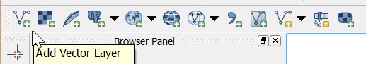
In newer versions of QGIS there is a single "add data" button that you can use.

Figure 8. Adding data in QGIS 3+

2.3. Import point data from text or spreadsheet

In many situations you might collect data in the field using a GPS, or get data from some other software (e.g., LSDTopoTools) that is not in a standard vector format. As long as the data has some spatial coordinates, you should be able to import it into QGIS. QGIS can read various formats but you will help yourself if you prepare your data in a common data format. Here we will describe importing data from either a spreadsheet (e.g., an .xlsx file) or a comma separated value file (.csv). One difference between ArcMap and QGIS is that ArcMap can import Excel files directly whereas in QGIS you need to convert to csv.

2.3.1. Preparing your text data or spreadsheet

These instructions refer to point data. Making polygons and lines requires information about how points are connected so we will not discuss that at this stage. For point data the key thing is to know where the points are! In the most common case one has collected data using a GPS, and written them down somewhere. We need to get these data into QGIS.

As we will see momentarily, QGIS asks for the X Field and Y Field. What these are will depend on the projection of your data.

If you are using a GPS you need to know what in which coordinate system the GPS reports its data. Make sure you check the settings of your GPS before you start collecting data so you know the coordinate system. If you fail to do this and the data is in latitude and longitude it is usually okay to assume the coordinates are in WGS84.

2.3.2. Geographic coordinates

If the coordinate system is geographic you will get latitude and longitude. This can be a little confusing because we often talk about x and y coordinates or latitude and longitude in that order, but in a sense these orders are reversed:
- The latitude is the Y Field
- The longitude is the X Field
If you get latitude and longitude, you might get them in degrees, minutes and seconds (e.g., 3° 10` 22``). I am afraid QGIS doesn’t really like this. You will need to convert to decimal degrees (e.g., 3.1727778). There are online converters for this. You can also just copy the coordinates in google maps and it will spit out the coordinates in decimal degrees.

2.3.3. Projected coordinates

If the coordinate system is projected, your data will either be in X, Y coordinates or Easting and Northing.
- Easting is the X Field
- Northing is the Y Field

2.3.4. Preparing the actual data in a spreadsheet

All you need to do is put your X and Y data in separate columns, and then have additional columns for the associated data. Here are two examples:

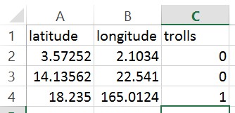Figure 9. Data in a spreadsheet with latitude and longitude coordinates

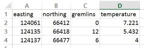Figure 10. Data in a spreadsheet with easting and northing
Hopefully you get the idea: you always need two columns for location data.
Now, you need to save spreadsheet data as a csv file (ArcMap can import xlsx or xls files directly but in QGIS it is easier to convert to csv). Simply take your spreadsheet and save as a csv file: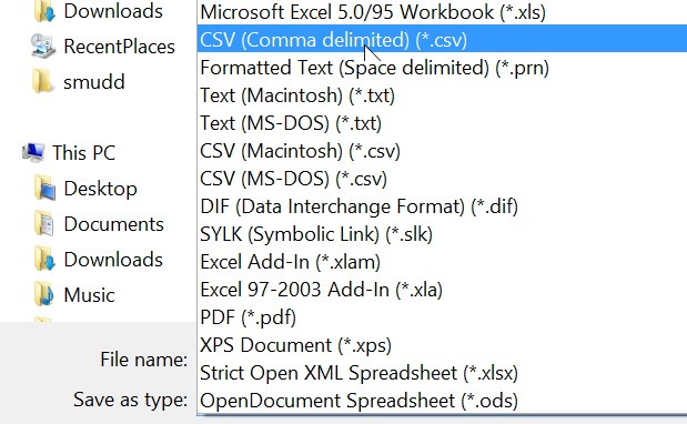

Figure 11. Save spreadsheet as csv
Once you’ve done this you can move on to the import data stage.

2.3.5. Preparing the actual data in a comma separated value (csv) file

A comma separated value file (csv) is just a text file that has values separated by commas. It does what it says on the tin. You can save any Excel worksheet as a csv file (see above). The advantage of csv files is that you don’t need Excel to read the data: you can read it with any text editor. However csv files only contain the values: you can’t save graphs or formatting. If you want separate worksheets you need to save them as separate files. The second example above in csv format look like this:

easting,northing,gremlins,temperature
124061,66412,0,7.221
124135,66418,12,5.432
124137,66477,6,4

2.3.6. A special case: GPS coordinates and the British National Grid

The British National Grid has a system of referencing that mixes letters and numbers, following the long British tradition of conceiving systems that are inscrutable to outsiders.

When you set your GPS to British National Grid, it will spit out some numbers but also some letters. For example, you might get something like NT 51422 13172. QGIS and other GIS systems only want numbers. How do we turn these letters into numbers?

The answers is that we need to count boxes along the grid, shown below:

Figure 12. Ordnance survey grid

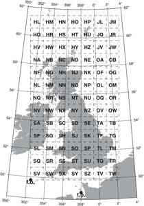
You need to add a digit to the front of your coordinates based on the letters. Each row and column represents a digit, and these are counted from the bottom left corner. The first row and column begin with digit 0, then next 1, and so on. The coordinate NT is in the 4th column and 7th row, but the first row and column are zero, so you put a 3 and 6 in front of the coordinates:

NT 51422 13172 → 351422, 613172

2.3.7. Another special case: csv data from LSDTopoTools

LSDTopoTools is a software package developed at the University of Edinburgh School of GeoScience for topographic analysis (if you want to use it, start here. You can also find full documentation). A number of its analysis routines create csv data. These data contain latitude and longitude coordiantes: these coordinates are in a WGS84 projection, EPSG:4326. When you import csv data from LSDTopoTools make sure your projections is EPSG:4326.

2.4. Importing the data into QGIS

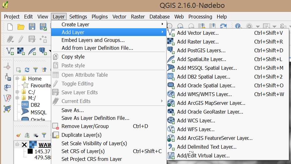
One you have organised your data, you can import it using the menus:

Layer→Add layer→Add Delimited Text Layer

Figure 13. Adding delimited layer

Once you select the Add delimited text layer option, you will get a dialog box asking to upload a file:

Figure 14. Add text layer dialog

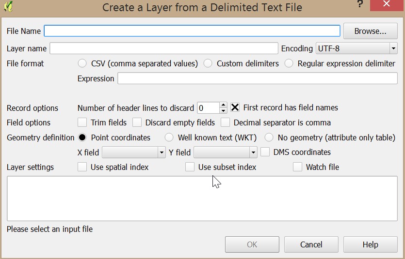
If you select the csv file you will see that many of the fields are selected for you automatically:

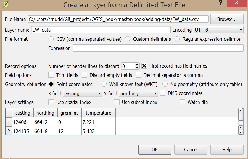
Figure 15. Add text once you have selected the file

You need to check on the X Field and Y Field entries to make sure that they are correct!

Another gotcha is that when loading a csv file you must select csv file format just below where you select the file.

Okay, nearly there!! Once you hit okay, you will need to select the coordinate system.

2.4.1. Selecting the coordinate system

This deserves its own header since it is so important. If you don’t choose the correct coordinate system, your data will be in the wrong place!! This is what the dialog looks like:

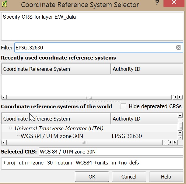
Figure 16. Selecting a coordinate system

In the image above, I have used the filter tool to select the WGS84 UTM 30N zone (this happens to be the zone for Scotland and much of western Europe). I found it using the EPSG code. Some common EPSG codes are listed in this table, and you can search for codes here: http://www.spatialreference.org/.

2.5. Saving your imported data

You can keep your data in csv format, but if you do that, you will need to import it each time you want to look at it. It is probably better to save it in a vector file format. Find the layer in the layers panel (in this example I have a layer called "Channel_width"), and right click on it. Then choose "save as":

Figure 17. Saving imported data

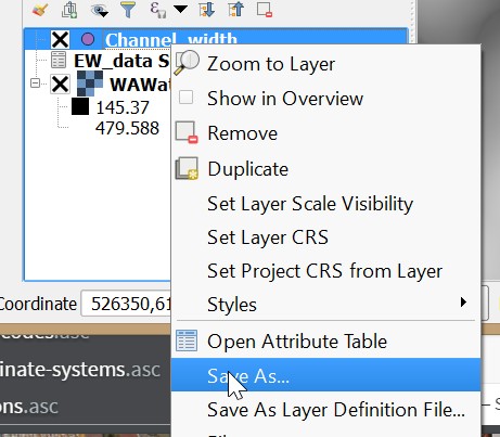
Once you have clicked "save as", you will get this dialog box:

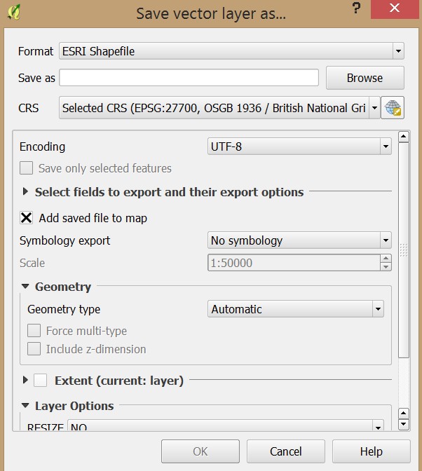
Figure 18. The dialog box for saving in vector format

The ESRI shapefile format is the default. This format can be read by a number of different software packages and is a safe choice. The drawback is that it generates many different files. Another option is the GeoJSON format, which is frequently used in web mapping applications. We recommend using one of these two formats.

QGIS is a bit picky about the file names when you save the file; you should use the "browse" dialog and name the file there rather than just typing a name.

You should notice that the new file has appeared in the layers dialog:

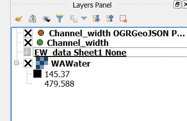
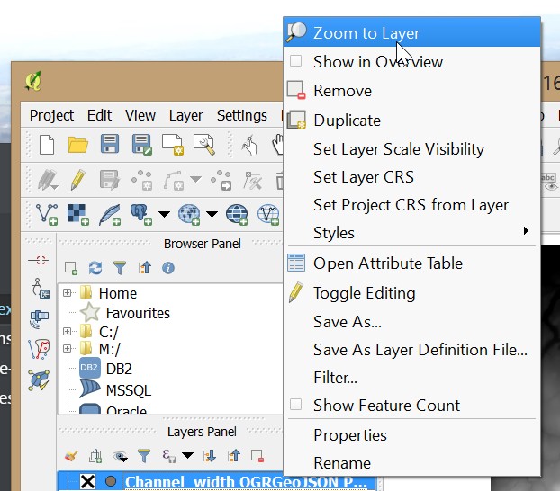
Figure 19. Your brand new vector data as a layer

You can now right click on the old layer (which is just csv data) and remove it. Note if you just want to zoom in on just your imported data, you can right click on the layer and select "zoom to layer":

Figure 20. Right click on a layer to zoom to its extent

2.6. Summary

By now you should be able to add data to QGIS.

3. Manipulating vector data

Occasionally you will need to adjust vector data, or add data categgories to your data based on other datasets.

3.1. Adjusting point locations

Handheld GPS units are often used in the field to determine location of sampling points. The accuracy of GPS measurements varies, and if you are working with a relatively high resolution DEM (e.g., 5 m resolution or better).

In this example we will look at some point data that was collected in a channel. We have extracted drainage area (using LSDTopoTools), in the image below the channels are those with high drainage area and have purple colours:

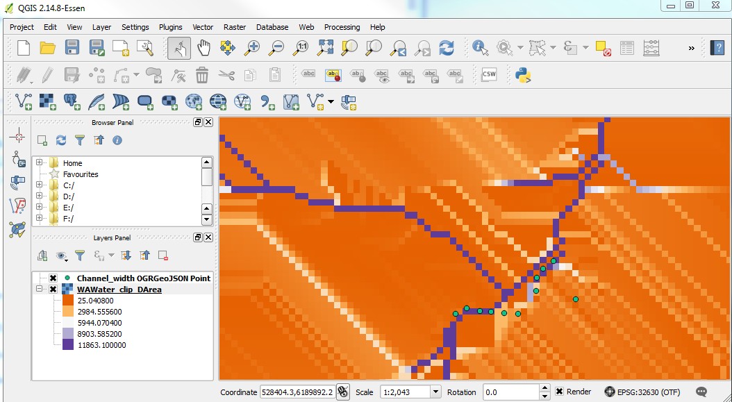
Figure 21. Point data aver drainage area

In this image, you can see that the channel point locations are not all on the channel. THis is because the DEM has a pixel size of 5 metres and the error on the GPS unit is greater than 5 metres. Also, in some cases the channel routing algorithms, combined with a noisy DEM, route the channels to the wrong place. In addition, one of these points seems spurious (the one anomalously to the East), so we might remove it from the dataset.

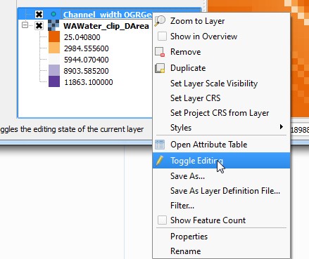
To edit the points, right click on the layer (not the csv file but a vector layer you created in previous steps) and select "toggle editing":

Figure 22. Enable editing of vector data

Once you do this the editing toolbar will become active:

Figure 23. The editing toolbar

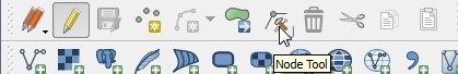
You can then select the "node tool" to move nodes to the channel. You can also delete nodes.

Figure 24. The node tool

You can either save or roll back edits (if you are unhappy with your work) by clicking on the icon with several pencils:

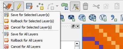
Figure 25. Saving or rolling back changes

Once you are finished editing make sure you turn the editing back off using the "toggle editing" button.

3.2. Extracting data from a raster onto points

Another common operation is to extract raster data onto points. There is a handy tutorial about this already: http://www.qgistutorials.com/en/docs/sampling_raster_data.html, but we are going to use the previous dataset here.

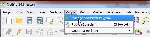
First, you need to click on the plugins menu bar and select "manage and install plugins":

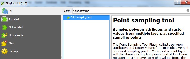
Figure 26. Opening the plugins browser

Search for "point sampling tool" and install:

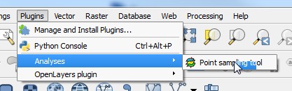
Figure 27. Get the point sampling tool

Once you do that, the "point sampling tool" can be found under the plugins menu:

Figure 28. Selecting the point sampling tool

Important notes about the point sampling tool

I have some bad news: the point sampling tool is very picky about the data you can use. Here are some gotchas:

If you edited your vector file and deleted a point, it turns out that point is still there, but has a "NULL" data entry. The extract point tool does not like this one bit. It is very hard to get rid of these points in a shapefile. In a geojson file, you can open the file, delete the point with "null" in the line, and save the file.
All of the layers need to be in the same projection. Because raster layers take up a lot of space you should check on your raster’s projection and then save your vector data in that same projection. Right click on the layer, select "save as" and then on the CRS button select the same projection as your raster.

Select the layer from which to extract data, and use the "browse" button to save the file. In addition, I recommend keeping all of the data in the original vector file:

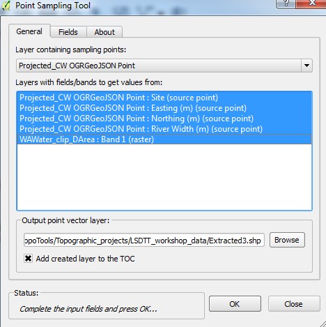
Figure 29. Extracting the data using the point sampling tool

The point extraction tool can only save files as ESRI shapefiles.

You can then right click on the new layer, view the attribute table and copy the data into a clipboard:

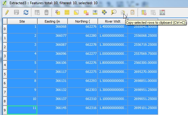
Figure 30. Copy the data to clipboard

This can then be pasted into a spreadsheet.

3.3. Selecting specific points

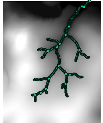
In this example we will load some data from csv and then select a subset of these points.

The data we will load comes from a chi analysis of a small Scottish catchement using LSDTopoTools. Note, chi is a Greek letter pronounced "kai".

First, we import the csv data. You should get something that looks a bit like this:

Figure 31. A chi network derived from LSDTopoTools

Now, suppose we only want a subset of these data. How do we extract them?

First, select the "select features by freehand" icon on the attributes toolbar (if this toolbar is missing, right click near the top of the QGIS window and activate it):

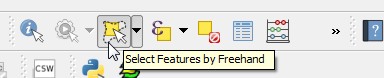Figure 32. Select features by freehand
Then, select the points you want:

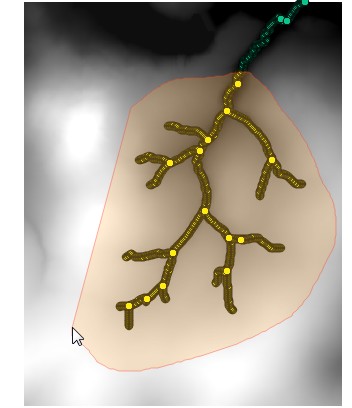Figure 33. Select the points you want
Right click on the layer, and then choose "save as". On the "save as" menu, make sure you select the option to "Save only selected features". In this case I am exporting a shapefile since I want access to the underlying data.

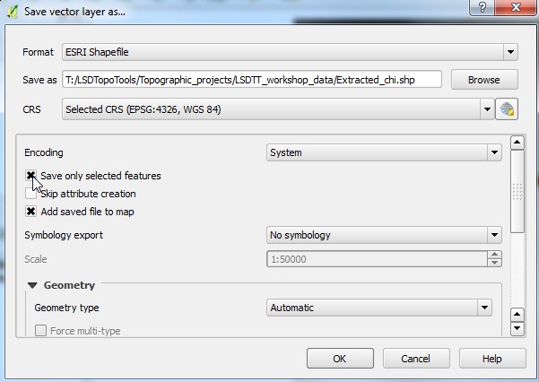Figure 34. Saving the selected features as a shapefile

You can also save as a csv file to just get the selected values. If you only want to plot, say, a river profile of selected points this can come in handy.
Great! Now you can make new files that include just a subset of your initial data.

3.4. Summary

In this chapter we have learned how to edit vector data, and extract underlying raster data using vector data.

4. More QGIS analysis using SAGA tools

We will continue working with data using the SAGA GIS tools that are embedded within QGIS.

We will add some data (more csv data, to give you more practise) and then look at subsampling this using a few new data layers.

4.1. First step: get topographic data

Before we begin, you will need some topographic data.
If you have installed LSDTopoTools, you will already have the data: it is called WA.bil, and is a DEM, from the Ordnance Survey, in a small catchment in the Lammermuir hills of Scotland.
If you haven’t got that data, go to this website: https://github.com/LSDtopotools/SmallExampleTopoDatasets
1. Click on the clone or download link, and download and unzip.
2. The relevant data is in the subdirectory BasicMetricsData.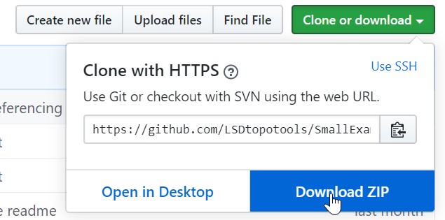
  
  Figure 35. Getting the example data

4.2. Adding a bit more data

First, find the example data (WA.bil) and add it to QGIS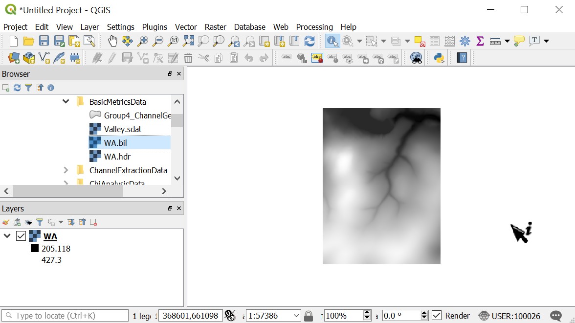

Figure 36. Add WA.bil to QGIS
Now we will add some data that is recorded as a csv in the British National Grid.

Here is the data (in comma separated value, csv, format):

False_Easting,False_Northing,Easting,Northing,AW 1
66222,61566,366222,661566,2.64
66165,61527,366165,661527,1.7
66195,61597,366195,661597,0.8
66161,61618,366161,661618,0.9
66154,61629,366154,661629,0.85
66144,61656,366144,661656,1.55
66129,61652,366129,661652,2.58
66102,61673,366102,661673,1.05
66095,61688,366095,661688,1
66046,61739,366046,661739,0.6

You can copy this into excel, and then use the text import wizard. Select "delimited" in the second window and delimit the data with a comma. You can then save this file as a csv file.
Now, import the data into QGIS using the Layer → add layer → add delimited text option. See the instructions for importing a csv. The data is in british national grid coordinates (EPSG:27700). Make sure that the X any Y coordinates are the Easting and Northing columns. False easting and false northing are the data spit out by a GPS in Britain. An explanation of why that is can be found << A special case: GPS coordinates and the British National Grid,earlier in this section>>.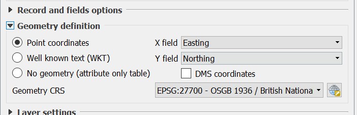

Figure 37. Adding data
The data should look like this:

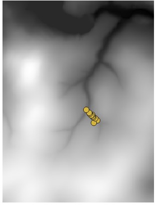Figure 38. Channel width data in the Whiteadder catchment
Okay, you are ready to move on to the next step.

4.3. Using the SAGA toolkit to process raster and other data

Now that we have a DEM (WA.bil) and some point data (that you imported with the last step), we are going to import some data using something called the SAGA toolkit. This contains a range of GIS functions embedded in QGIS.
To get to the toolkit, use the Processing→toolkits menu button in QGIS: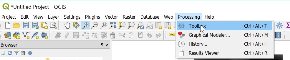

Figure 39. The toolkits button in QGIS
Once you do this, you will get a huge number of options:

Figure 40. The toolkits available in QGIS (newer versions will have even more options)
There are loads of SAGA options. Lets use the valley depth option: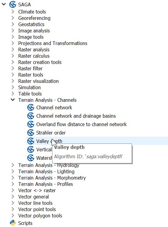

Figure 41. SAGA valley depth option
Save the valley depth as a file in the same directory as your DEM

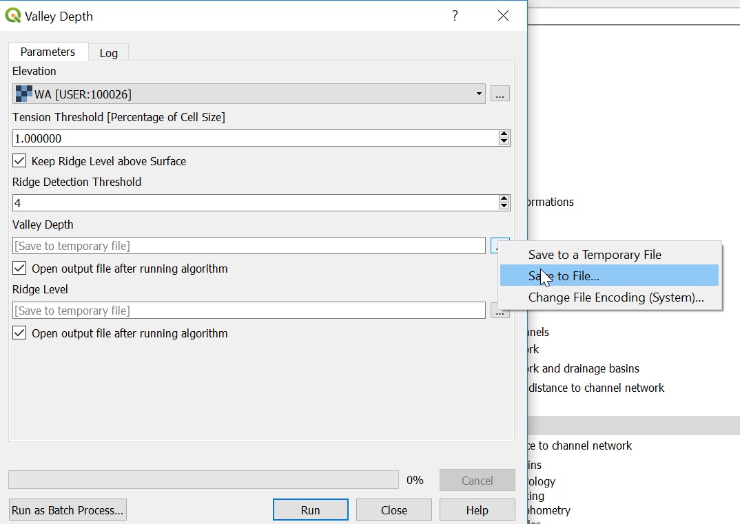Figure 42. Save valley depth
Running this routine will take some time. You can only save this as a articular SAGA file.
You will end up with some data that looks like this:

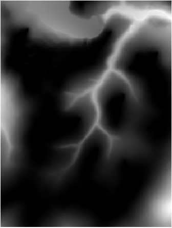Figure 43. Valley depth in the Whiteadder catchment

4.4. Sampling rasters with the SAGA toolkit

Okay, now we have some valley depth data! Lets add that to our channel width data.
Actually, we need to do something first. SAGA outputs data in its own idosyncratic data format that is badly georeferenced. So when you try to do subsequent analysis it might break things. For point extraction, it is essential that the data layers are in the same projection.
1. First, export the valley depth raster:
  
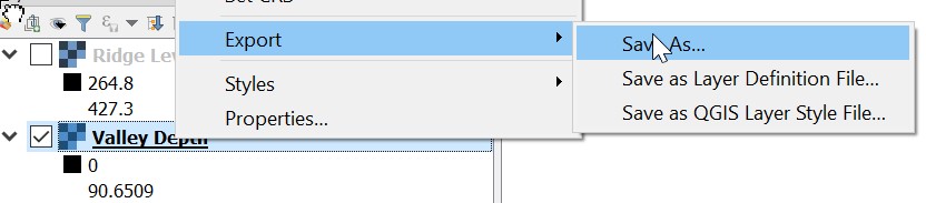  Figure 44. Export the SAGA layer to a different file format
2. In this particular case, the main raster (WA.bil) is in UTM zone 30 (EPSG:32630) so put the new DEM in this coordinate system: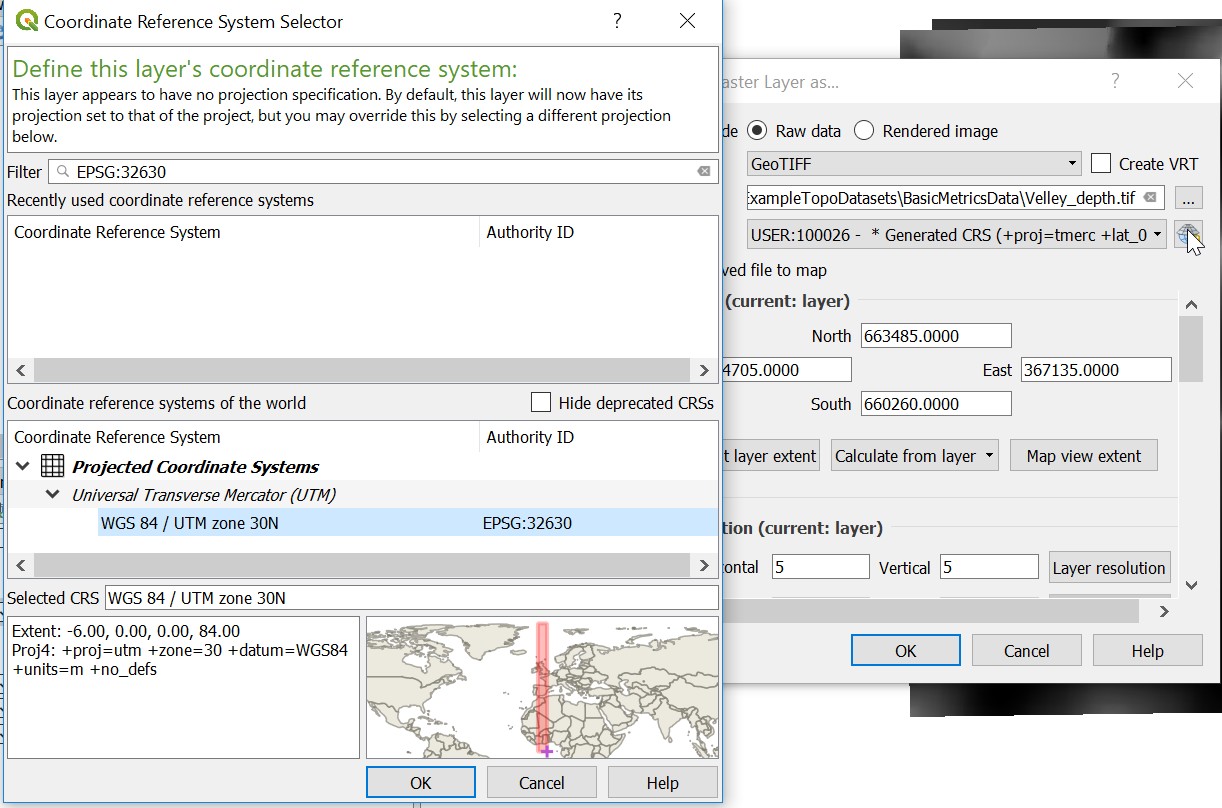
  
  Figure 45. Ensure you have the same eoreferencing as the base DEM

Okay, you should also save the csv data as a shapefile, and it is probably clever to put it in this same coordinate system (do the same thing: right click on the data layer and use export tool).

This tool is very sensitive to coordinate systems. It will not like it if any of your data is in a different coordinate system. So make sure that all your layers are projected in the same way!

Now we can move on to the SAGA option for sampling rasters.

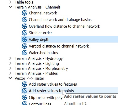Figure 46. Sample points using SAGA
When you do this make sure to add the grids that you want to sample. It looks like you can add loads of rasters! Unfortunately, testing suggest it will only actually add one raster at a time. Note that each layer has its projection listed. You should only choose layers with the same EPSG code.

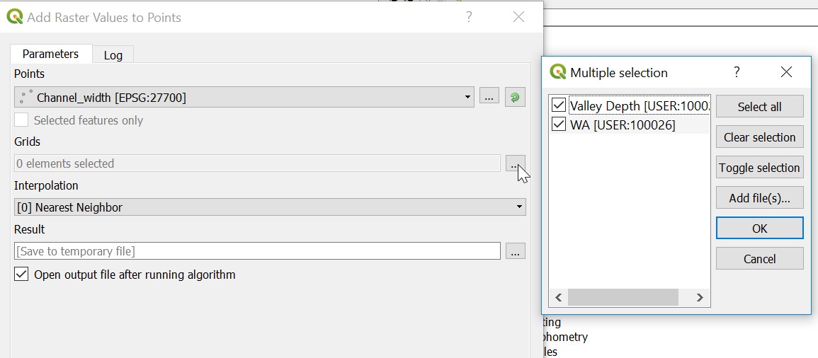Figure 47. Options for sampling points using SAGA
Also make sure to save the output. And make sure you sample using either bilinear or cubic: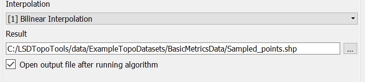

Figure 48. More options for sampling points using SAGA
You will get a points layer in the same location, but if you look at the data by right clicking on the layer and opening the attribute table:

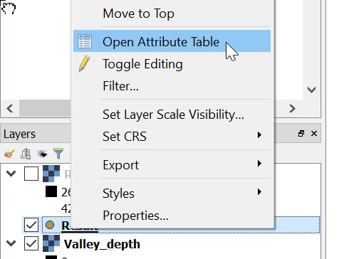Figure 49. Open an attribute table

You will then see the raster data in a table:

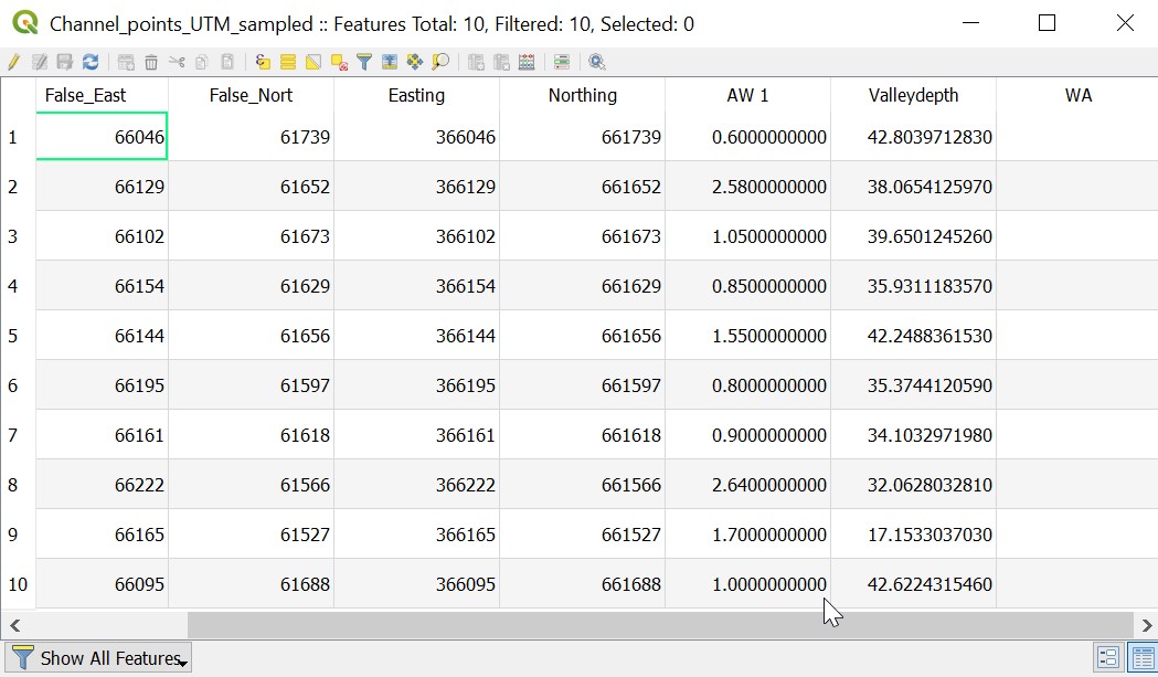Figure 50. The attributes
You can export this to an excel spreadsheet or csv if you wish.

4.5. Summary

You now should have some familiarity with the SAGA GIS tools within QGIS and should feel confident to explore the options.

5. An example using data from LSDTopoTools

This chapter gives and example of computing some basic raster and csv data from LSDTopoTools and then importing it into QGIS. We use these examples in of one the practical exercises in the University of Edinburgh course, Eroding Landscapes.

One of the objectives of this exercise is to get you familiar with moving between a linux environment and QGIS.

5.1. Generating the data

Okay, I am afraid this is something of a bait and switch: we are going to generate data using LSDTopoTools and to do that you need to follow the instructions for basic LSDTopoTools usage.

At the end of that excercise you should

Have LSDTopoTools installed.
Be able to get into a linux environment (using University of Edinburgh servers and MobaXterm, or using Docker on your own computer).
Have run the initial lsdtt-basic-metrics commands from the examples.

A few linux shortcuts

pwd — Tells you what directory you are currently in.

cd — change directory. You need to give it the directory name.

cd .. — go up a directory.

ls — list what is in the directory.

mkdir — make a new directory.

wget — download a file from the internet. Needs to be followed by an html/ftp address.

5.1.1. What data should you have and where is it?

After running the basic LSDTopoTools usage, you will have a bunch of datasets within a directory called LSDTT_workshop_data. If you followed the instructions it will be inside a directory called LSDTopoTools.

In your host operating system (e.g., the Windows computer in the Edinburgh computer labs and not the Linux machine you have accessed through MobaXterm), use your file explorer to find all these files.
We are going to look at these using QGIS.

5.2. A first basic analysis

In the first example you generated a hillshade.
Open QGIS and load the raster. The new raster is in the same directory with your other data and is called WA_FirstExample_hs.bil. To load raster data in QGIS follow these instructions: Adding raster data. The data will look like this: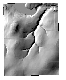

Figure 51. A hillshade of the Whiteadder catchement
As you can see, the DEM has quite a few artifacts. There isn’t much we can do about that, I’m afraid.

5.3. Getting surface metrics

The second example generated a number of surface fitting rasters. These all have secondexample in the filename.
In this case the program is printing slope, aspect, curvature, and tangential curvature rasters. They have filenames that reflect their contents so have a look. Slope tells you how steep the landscape is, aspect which direction the surface is pointing, curvature how, uh, curvy the landscape is (mathematically it is how quickly slope changes in space) and the tangential curvature is how curvy the landscape is in the direction of steepest descent. Essentially tangential curvature tells you how tightly curved contours are and is useful for finding valleys.
The way these are calculated is by fitting a surface of radius surface_fitting_radius to the points in the DEM and then calculating derivatives of that surface.
Load these into QGIS.

5.3.1. Questions and tasks for surface metrics

Try changing the surface_fitting_radius using lsdtt-basic-metrics. What happens?

5.4. Draniage area and channel extraction

If you run the WA_BasicMetrics03.driver you will get a channel network, and some additional rasters.
The channel network is stored as a csv file, WA_ThirdExample_CN.csv.
To load this in QGIS, follow the instructions here: Import point data from text or spreadsheet. You will get something that looks a bit like this:

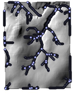Figure 52. A simple channel network

5.4.1. Questions for channel extraction.

Try changing the threshold_contributing_pixels parameter. What happens to the channel network.
More advanced: You can get a smoothed elevation raster with the following driver file line: print_smoothed_elevation: true. Try creating a smoothed elevation raster and then using this smoothed raster for the drainage extraction. You will need to change the read_fname: parameter to reflect the smoothed raster.

5.5. Sampling a raster with point data.

In many cases you might want to get some data from your raster to map nto some points you collected either in the field or extracted from a DEM (for example, like your channel network).

One way to do this is by using the QGIS point sampling tool. However, that tool is tempermental and we have another way to do that using LSDTopoTools.

We have added a driver function that extracts information from a raster and adds it to a csv.
You can run it jusgt as you ran the previous basic analyses using the parameter file WA_BasicMetrics07.driver.

This is what the paramete file looks like:

# Parameters for burning data
# You need to run the Third Example before running this example to get the channel network CSV
# Comments are preceeded by the hash symbol
# Documentation can be found at: https://lsdtopotools.github.io/LSDTT_documentation/LSDTT_basic_usage.html

# These are parameters for the file i/o
read fname: WA
write fname: WA_SeventhExample
channel heads fname: NULL

# Convert to json
convert_csv_to_geojson: true

# Raster burning
burn_raster_to_csv: true
burn_raster_prefix: WA_ThirdExample_d8_area
burn_data_csv_column_header: d8_area
csv_to_burn_name: WA_ThirdExample_CN.csv

The key information is at the end.
1. burn_raster_to_csv: this switches on the "burning" or data from a raster to a csv file.
2. burn_raster_prefix: this is the name of the raster whose data you want on the csv. Don’t include the extension (e.g., bil)
3. burn_data_csv_column_header: this is what you will call the new column in your csv. It could be anything, so choose wisely!
4. csv_to_burn_name: This is the name of the csv file you want to append with the data from the raster.

You csv needs to have lat-long coordinates in WGS84 (EPSG:4326)

5.5.1. Questions:

Try to change the raster from which you extract data.
Try to do the analysis mulpiple times to get multiple raster datasets on your csv file.
Try to make your own csv to burn to the raster.
1. First, create a csv with headers latitude and longitude (separated by a comma).
2. Then go into google maps and right click in the Whiteadder catchement, selecting "what’s here"?
3. Use the lat long coordinates to enter into your csv, save it, and try to burn raster values to it.

5.6. Channel steepness using chi analysis

In a final example, we will extract some channel steepness metrics. We will be using chi analysis, the purpose of which is to normalise channel profiles for drainage area. See the following paper for details: https://onlinelibrary.wiley.com/doi/full/10.1002/esp.3302

We will use a program within LSDTopoTools to do the chi transformation and look at the steepness of the channel. The method is descripbed in this paper: https://agupubs.onlinelibrary.wiley.com/doi/10.1002/2013JF002981

5.6.1. Run the chi example

If you have followed the instructions for installing LSDTopoTools you will already have the required program.

Go into the directory with the example data from the previous examples.

Run the following command:

$ lsdtt-chi-mapping WA_ChiMapping01.driver

This is a different program from the last example (lsdtt-chi-mapping) but the parameter file has the same format:

# Parameters for extracting simple surface metrics
# Comments are preceeded by the hash symbol
# Documentation can be found at: https://lsdtopotools.github.io/LSDTT_documentation/LSDTT_basic_usage.html

# These are parameters for the file i/o
read fname: WA
write fname: WA_ChiFirstExample
channel heads fname: NULL

# Some basin selection parameters
only_take_largest_basin: true
find_complete_basins_in_window: false
print_basin_raster: true

# We only want the study basin so I have selected the elevation of its outlet
minimum_elevation: 218

# Now the chi analysis
print_segmented_M_chi_map_to_csv: true
print_chi_data_maps: true
convert_csv_to_geojson: true

If you have looked at LSDTopoTools parameter files before, some of this will look familiar to you.
This will spit out four files (two geojson and two csv): WA_ChiFirstExample_MChiSegmented and WA_ChiFirstExample_chi_data_map.

==== Looking at channel steepness data
The WA_ChiFirstExample_MChiSegmented files contain channel steepnesses. If we load the geojson file it will look like this: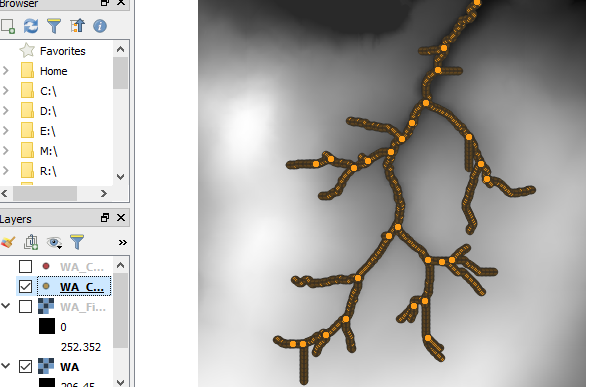

Figure 53. A channel network from chi analysis
If you click on the data you will see it has loads of different data elements. One of these is m_chi. This is the channel steepness. Because this was run with A_0_ = 0, m_chi is the same as the channel steepness index, k_sn_.
You can right click on this layer, and select properties.

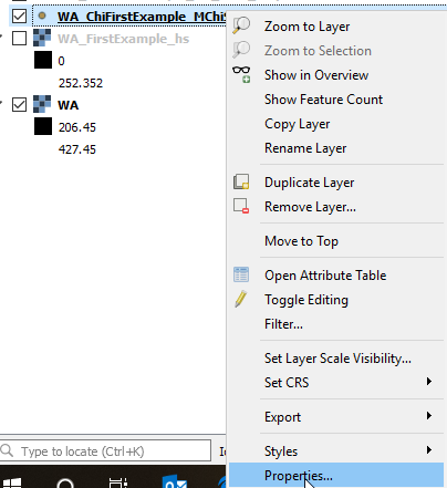Figure 54. Selecting point properties
Then click on the symbology tab:

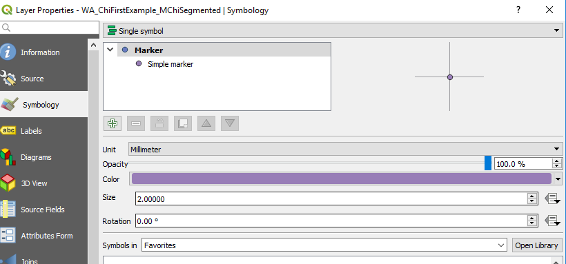Figure 55. Selecting symbology
And then click on graduated:

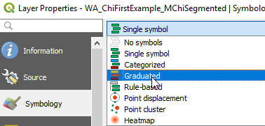Figure 56. Graduated colours
And then select the m_chi as the data element by which to colour. You MUST click on the Classify button below for this to work:

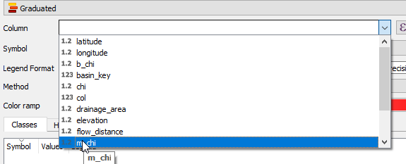Figure 57. Colour by M_chi_
You should end up with a plot that looks a bit like this:

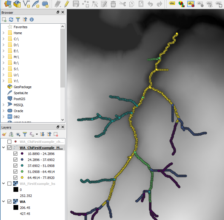Figure 58. Channel steepness map

5.7. Summary

You now have seen the basic interface of LSDTopoTools programs, got a small taste of Linux, and know a few things about QGIS. From here you should be able to move on to more advanced topographic analysis.

Appendix A: Projections and transformations

We live on the surface of a planet, Earth, that is almost a perfect sphere. Our computer screens and sheets of paper are flat. This causes all sorts of problems. The problems are addressed by using map projections. I am afraid if you use geographic data you will have to deal with projections, which, unless you are a cartographer, will be tedious and frustrating. Hopefully this appendix will help you understand how to appropriately manage projections within QGIS and other environments.

A.1. What are coordinate systems?

Coordinate systems are simply reference frames for describing position. All geographic data must be placed in a coordinate system. Over the years, cartographers have developed numerous systems so now whenever we collect geographic data there are a myriad of choices when it comes to selecting a coordinate system. A full description can be found on the ESRI website, so here we will stick to the basics.

Firstly, a coordinate system can fall into two categories:

A geographic coordinate system which uses spherical coordinates. Latitude and longitude are the most familiar measures of such a coordinate system since these give locations on the surface of a sphere. The units of geographic coordinate systems are angular units (e.g., degrees).
A projected coordinate system projects your data, collected from the surface of a sphere, onto a flat surface. National grids (like the British National Grid) tend to be in projected coordinates: they measure locations in distances (e.g., metres from a reference location, sometimes reported on easting and northing).

There are many, many different coordinate systems. For example, in the United States there are 124 (!!) local coordinate systems called State planes. Most countries have their own coordinate system. There are also global coordinate systems.

A.2. Common EPSG codes

You can search for coordinate systems on the handy http://spatialreference.org/ website.

Table 1. Common EPSG codes
EPSG code	Coordinate system
EPSG:4326	WGS1984 Global Geographic coordinate system.
EPSG:326XX	WGS1984 Universal Transverse Mercator (UTM) for the northern hemisphere. A global projected coordiante system. The XX above denotes the zone. Here is an image of the zones.
EPSG:327XX	WGS1984 Universal Transverse Mercator (UTM) for the southern hemisphere. A global projected coordiante system. The XX above denotes the zone. Here is an image of the zones.
EPSG:3857	Web Mercator projected coordinate system (used in Google maps and Open Street Map)
EPSG:27700	The British National Grid