1. Introduction
Terrestrial landscapes are almost all dissected by channels. Mapping channels and rivers has been a feature of cartography from its start. A few centuries ago, finding river sources use to be an amusing way to get your name in a newspaper. In fact, there continue to this day to be stunts looking for the source of major rivers.
Taking boats through precarious jungles is good fun for some, but in fact we can now use digital topography to look for the characteristic topographic signs of channels on the landscapes using remotely-sensed data. These signs can simply be the "v-shaped" valleys that you might have learned about in school, or could include more advanced techniques. We now have topographic data covering the entire planet so as long ago as 2005 (when the SRTM 90 dataset was released) it was trivially easy to find the longest channel in a river network. Knowing in detail where the channel head is, however, is not at all trivial and now that lidar data is widely available, we can look for topographic signature of channel at scaled approaching those of the actual channel heads.
In this documentation we have compiled several methods for determining the location of channel heads using high resolution data, and ported them into LSDTopoTools. These algorithms should be, for the most part, accurate to ~20-30 metres of the actual channel head. For details see the following paper:
We have also attempted to quantify the resolution of data needed for the different methods; the answer is that you might be able to extract a reasonable channel network from 10 metres resolution data, but 30 metre resolution data is not trustworthy. If you have lidar data, use that. The details are contained in the following paper:
For completeness we include our historic functions for calculating channel sources, but in general the only tool you will need is The Channel Extraction tool. We also refer readers to the GeoNet channel extraction tool, which was developed by Paola Passalacqua and colleagues.
2. Get the code for channel extraction
Channel extraction is included within the LSDTopoTools package.
2.1. Installation of the channel extraction algorithms
-
Good news! If you have installed LSDTopoTools, you already have the channel extraction tools.
-
In you haven’t installed it, follow the LSDTopoTools installation instructions.
-
The channel extraction code is called
lsdtt-channel-extraction.
2.2. Example datasets
We have provided some example datasets which you can use in order to test the channel extraction algorithms. In this tutorial we will work using a lidar dataset from Indian Creek, Ohio.
2.2.1. Get the test data
If you have followed the installation instructions and grabbed the example data, you already have what you need! If not, follow the steps below:
-
If you are using a docker container, just run the script:
# Get_LSDTT_example_data.sh -
If you are on a native linux or using the University of Edinburgh servers, do the following:
-
If you have installed LSDTopoTools, you will have a directory somewhere called
LSDTopoTools. Go into it. -
Run the following commands (you only need to do this once):
$ mkdir data $ cd data $ wget https://github.com/LSDtopotools/ExampleTopoDatasets/archive/master.zip $ unzip master.zip $ mv ./ExampleTopoDatasets-master ./ExampleTopoDatasets $ rm master.zip -
WARNING: This downloads a bit over 150Mb of data so make sure you have room.
-
The datasets for our channel extraction tests are in the subdirectory /LSDTopoTools/data/ExampleTopoDatasets/ChannelExtractionData in the Docker container.
There are several datasets within this directory, for the initial tutorial we will focues on the Indan Creek, Ohio DEM. It is in the subdirectory IndianCreek_1m
3. The Channel Extraction tool
Our channel extraction tool bundles four methods of channel extraction. These are:
-
A rudimentary extraction using a drainage area threshold.
-
A geometric method combining elements of Geonet (Passalacqua et al., 2010) and Pelletier (2013) methods that we developed for Grieve et al. (2016) and Clubb et al. (2016) We call this the "Wiener" method (after the wiener filter used to preprocess the data).
These methods are run based on a common interface via the program lsdtt-channel-extraction.
3.1. Starting up LSDTopoTools and getting the channel extraction tool
-
The channel extraction tool (
lsdtt-channel-extraction) is included in LSDTOpoTools, so if you have installed LSDTopoTools you will aready have what you need.-
If you haven’t installed LSDTopoTools, follow the LSDTopoTools installation instructions).
-
-
Before you do anything, you need to start an LSDTopoTools session.
-
If you are using Docker , start the container:
$ docker run -it -v C:\LSDTopoTools:/LSDTopoTools lsdtopotools/lsdtt_pcl_docker -
Then run the start script.
# Start_LSDTT.sh
-
-
If you haven’t got the example data yet, run:
# Get_LSDTT_example_data.sh -
If you are using native linux, read the LSDTopoTools installation instructions.
Like most of LSDTopoTools, you run this program by directing it to a parameter file. The parameter file has a series of keywords. Our convention is to place the parameter file in the same directory as your data.
3.1.1. Running a typical lsdtt-channel-extraction analysis
In the next section we will walk you though an analysis. However, reading this will help you understand where you are going, so we recommend you read the whole thing!
-
You run the program from a terminal window
-
You can supply the program with:
-
a directory name
-
a parameter file name
-
both of these things
-
none of these things
-
-
If you don’t supply a parameter filename, the program will assume the parameter file is called
LSDTT_parameters.driver -
If the parameter file doesn’t exist, you will get an error message.
Any of the following calls to one of the programs will work, as long as your files are in the right place:
$ lsdtt-channel-extraction $ lsdtt-channel-extraction /LSDTopoTools/data/A_project $ lsdtt-channel-extraction AParameterFile.param $ lsdtt-channel-extraction /LSDTopoTools/data/A_project AParameterFile.param -
The program name (
lsdtt-channel-extraction), the directory name (/LSDTopoTools/data/A_project) and the parameter file name (AParameterFile.param) will change but all LSDTopoTools calls follow this same basic structure.
3.2. First Example of channel extraction.
-
We are going to extract a channel networks from Indian Creek, a small creek in Ohio. It was using in the study Clubb et al., 2014.
-
Once you have run
Start_LSDTT.shyou are ready to run an analysis. -
Go into the directory containing the Indian Creek DEM. In the Docker container it is here:
# cd /LSDTopoTools/data/ExampleTopoDatasets/ChannelExtractionData/IndianCreek_1m -
Now run the channel extraction code:
# lsdtt-channel-extraction IndianCreek_example01.param -
The parameter file looks like this
# These are parameters for the file i/o read fname: indian_creek channel heads fname: NULL # Parameter for filling the DEM min_slope_for_fill: 0.0001 # Parameters for selecting channels and basins threshold_contributing_pixels: 1000 print_area_threshold_channels: true write_hillshade: true -
This will generate a very basic channel network where channels begin where the contributung pixels are greater than the parameter
threshold_contributing_pixels. -
If you set a channel extraction method to true (in this example,
print_area_threshold_channels: true), you will get two files:-
A file with the extension
sources.csv: This has the location of the source pixels. We describe the file format below. -
A file with the extension
CN.scv: This contains the channel network, along with the Strahler order of the channels.
-
-
If you want to know the file formats, please see the [channel extraction appendix for file formats]
-
In addition, we set
write_hillshade: true, so we also get a hillshare raster, denoted by theHSin the filename. -
The channel networks and sources are in csv format, which foes not retain georeferencing information. That means, when you load it into a GIS, you will need to tell the link:LSDTT_QGIS.html#_another_special_case_csv_data_from_lsdtopotools [GIS what projection you are using].
-
If you want a file that can be directly read into a GIS, then use the parameter
convert_csv_to_geojson: true
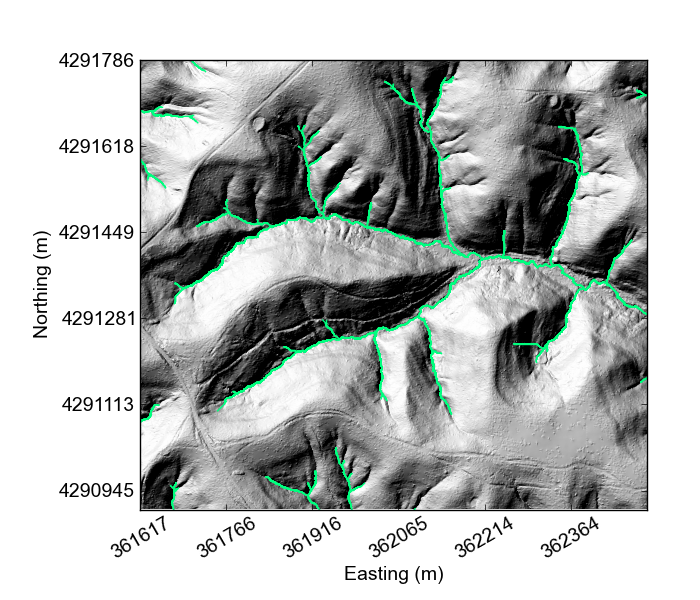
The figure below shows the extracted channel network for the Indian Creek field site with a threshold of 1000 pixels (which works out to 1000 m2 because it is a 1 m resolution DEM).
3.3. More complex channel extraction
For higher-resolution DEMs a number of different methods have been developed to extract channel networks more accurately. This section details how to extract channels using methods relying on geometric signatures of channel incision, primarily how it affects planform curvature. Although many methods have been developed that use a variety of planform curvature to detect channel heads from high resolution topogrpahy (e.g., GeoNet, which was developed by Paola Passalacqua and colleagues) , we will use the three methods available in lsdtt-channel-extraction
| Name | paramter file keyword | Notes |
|---|---|---|
Pelletier |
|
A method developed by Pelletier (2013) and implemented in LSDTopoTools that uses spectral filtering and tangential curvature. |
Wiener |
|
A method that combines some elements of the Pelletier method and some of the GeoNet method that is available within LSDTopoTools. It was described by Grieve et al., ESURF, 2016. In that study it was found to be the least sensitive to grid resolution. We call this the Wiener method since it is based on a Wiener spectral filter (the Pelletier method also uses this filter). |
Driech |
|
The Dreich method that aims to find channel heads by looking at the break in the properties of topographic profiles that occur when fluvial incision gives way to hillslope sediment transport processes. It is different from the geometric methods described above in that it looks for a theoretical signal of fluvial incision rather than the planform curvature of the landscape. |
The method you use should be chosen based on the particular aims of your study: if you only want a single channel network we suggest the Wiener method (see Grieve et al., ESURF, 2016 and Clubb et al., WRR, 2014), but because the Dreich method takes a totally different aproach to identifying channels it can be useful to compare the networks generated by these two methods to get an estimate of the uncertainty in the network extent.
3.3.1. Switching on the high resolution extraction methods
-
We are staying at Indian Creek. However, this time you will run the second parameter file:
# lsdtt-channel-extraction IndianCreek_example02.paramThis takes a lot longer than the threshold area method! It takes around 22 minutes on my laptop. -
The parameter file looks like this
# These are parameters for the file i/o read fname: indian_creek channel heads fname: NULL # Parameter for filling the DEM min_slope_for_fill: 0.0001 # Parameters for selecting channels and basins threshold_contributing_pixels: 1000 connected_components_threshold: 100 print_area_threshold_channels: false print_wiener_channels: true print_pelletier_channels: true print_dreich_channels: true -
You will get both
sourcesandCNfiles for each of these methods. -
The
connected_components_thresholdis the minimum number of connected pixels to create a channel. 100 is the default and for most applications you can leave this alone.
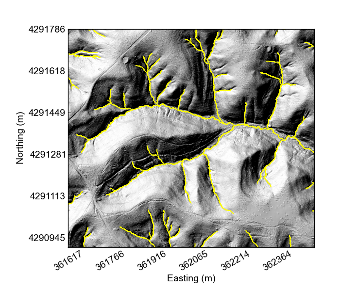
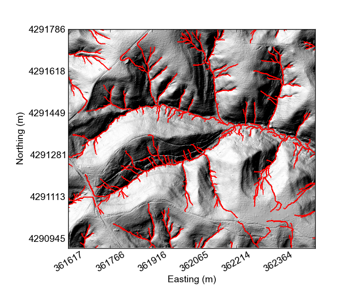
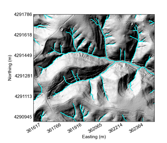
The figures below show the extracted channel network for the Indian Creek for the three different methods.
4. Calculating drainage density
Drainage density is a fundamental landscape metric which describes the total length of channels in a basin normalised by the basin area, first described by Horton (1945). In this chapter we describe how to calculate the drainage density and mean hilltop curvature of a specified order of drainage basins (for example, all second order basins). We also include code which will calculate the drainage density of each basin given a list of cosmogenic radionuclide (CRN)-derived erosion rate data. We used this code to examine the relationship between drainage density and erosion rate in our paper published in JGR Earth Surface in 2016.
Citation: Clubb, F. J., S. M. Mudd, M. Attal, D. T. Milodowski, and S. W. D. Grieve (2016), The relationship between drainage density, erosion rate, and hilltop curvature: Implications for sediment transport processes, J. Geophys. Res. Earth Surf., 121, doi:10.1002/2015JF003747.
4.1. Get the code for drainage density analysis
The code for the drainage density analysis can be found in our GitHub repository. This repository contains code for extracting the drainage density for a series of basins defined by points from cosmogenic radionuclide samples, as well as the drainage density and mean hilltop curvature for basins of a specified order.
4.1.1. Clone the GitHub repository
First navigate to the folder where you will keep the GitHub repository. If you have downloaded LSDTopoTools using vagrant, then this should be in the folder Git_projects. Please refer to the documentation on installing LSDTopoTools. To navigate to this folder in a UNIX terminal use the cd command:
vagrant@vagrant-ubuntu-precise-32:/$ cd /LSDTopoTools
vagrant@vagrant-ubuntu-precise-32:/$ cd /Git_projects
You can use the command pwd to check you are in the right folder. Once you are in this folder, you can clone the repository from the GitHub website:
vagrant@vagrant-ubuntu-precise-32:/LSDTopoTools/Git_projects$ pwd
/LSDTopoTools/Git_projects
vagrant@vagrant-ubuntu-precise-32:/LSDTopoTools/Git_projects$ git clone https://github.com/LSDtopotools/LSDTopoTools_DrainageDensity.git
Navigate to this folder again using the cd command:
$ cd LSDTopoTools_DrainageDensity/4.1.2. Alternatively, get the zipped code
If you don’t want to use git, you can download a zipped version of the code:
vagrant@vagrant-ubuntu-precise-32:/LSDTopoTools/Git_projects$ pwd
/LSDTopoTools/Git_projects
vagrant@vagrant-ubuntu-precise-32:/LSDTopoTools/Git_projects$ wget https://github.com/LSDtopotools/LSDTopoTools_DrainageDensity/archive/master.zip
vagrant@vagrant-ubuntu-precise-32:/LSDTopoTools/Git_projects$ gunzip master.zip
GitHub zips all repositories into a file called master.zip,
so if you previously downloaded a zipper repository this will overwrite it.
|
4.1.3. Get the example datasets
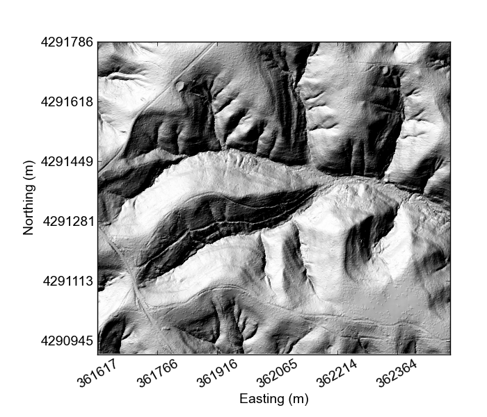
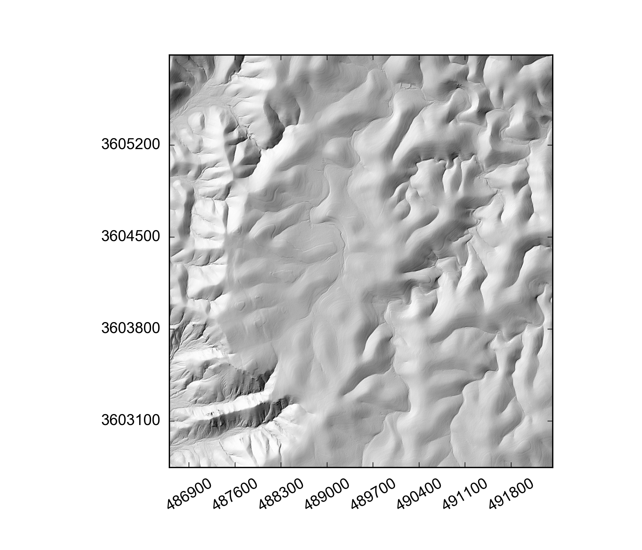
We have provided some example datasets which you can use in order to test the drainage density analysis. In this tutorial we will work using a LiDAR dataset from the Guadalupe Mountains, New Mexico. This is a clip of the original dataset, which we have resampled to 2 m resolution. The full dataset is available from OpenTopography.. If you are using the vagrant distribution, create a new folder within the Topographic_projects folder, and then navigate to this folder:
vagrant@vagrant-ubuntu-precise-32:/LSDTopoTools/Topographic_projects$ mkdir Guadalupe_NM
vagrant@vagrant-ubuntu-precise-32:/LSDTopoTools/Topographic_projects$ cd Guadalupe_NM/
You can get the clip from our ExampleTopoDatasets repository using wget:
$ wget https://github.com/LSDtopotools/ExampleTopoDatasets/raw/master/Guadalupe_DEM.bil
$ wget https://github.com/LSDtopotools/ExampleTopoDatasets/raw/master/Guadalupe_DEM.hdr
This dataset is already in the preferred format for use with LSDTopoTools (the ENVI bil format). The figure below shows a shaded relief map of part of the Guadalupe Mountains DEM which will be used in these examples.
4.1.4. Get the example parameter files
We have also provided some examples parameter files that are used to run the drainage density analysis. These should be placed in the same folder as your DEM (e.g. in the folder /LSDTopoTools/Topographic_projects/Guadalupe_NM/. You can get the example parameter file using wget:
$ wget https://github.com/LSDtopotools/ExampleTopoDatasets/tree/master/example_parameter_files/drainage_density_guadalupe.driver4.1.5. Python scripts
We have also provided some Python scripts for creating figures from the draiange density analysis. These should produce similar figures to those in Clubb et al. (2016), JGR-ES. These scripts are in the directory Python_scripts within LSDTopoTools_DrainageDensity:
vagrant@vagrant-ubuntu-precise-32:/LSDTopoTools/Git_projects/LSDTopoTools_DrainageDensity$ cd Python_scripts
vagrant@vagrant-ubuntu-precise-32:/LSDTopoTools/Git_projects/LSDTopoTools_DrainageDensity/Python_scripts$ ls
drainage_density_plot.py	drainage_density_plot_cosmo.py
4.2. Preliminary steps
4.2.1. Getting the channel head file
Before the drainage density analysis can be run, you must create a channel network for your DEM. This can be done using any of the channel extraction algorithms within LSDTopoTools. Once you have run the channel extraction algorithm, you must make sure that the bil and hdr files with the channel head locations are placed in the same folder as the DEM you intend to use for the drainage density analysis.
4.2.2. Selecting a window size
Before we can run the drainage density algorithm, we need to calculate the correct window size for calculating mean hilltop curvature across the DEM. Please refer to the selecting a window size section for information on how to calculate a window size for your DEM.
4.3. Analysing drainage density for all basins
This section provides instructions for how to extract the drainage density and mean hilltop curvature for every basin in the landscape of a given order (e.g. all second order drainage basins).
4.3.1. Creating the paramter file
In order to run the drainage density analysis code you must first create a parameter file for your DEM. This should be placed in the same folder as your DEM and the channel heads bil file. If you followed the instructions in the Get the code for drainage density analysis section then you will already have an example parameter file for the Guadalupe Mountains DEM called drainage_density_guadalupe.driver. Parameter files should have the following structure:
Name of the DEM without extension
Name of the channel heads file - will vary depending on your channel extraction method
Minimum slope for filling the DEM
Order of basins to extract
Window size (m): calculate for your DEM resolution
An example parameter file for the Guadalupe Mountains DEM is set out below:
Guadalupe_DEM
Guadalupe_DEM_CH_DrEICH
0.0001
2
6
4.3.2. Step 1: Get the junctions of all the basins
The first step of the analysis creates a text file with all the junction numbers of the basins of the specified stream order. Before the code can be run, you must compile it using the makefile in the folder LSDTopoTools_DrainageDensity/driver_functions_DrainageDensity. Navigate to the folder using the command:
$ cd driver_functions_DrainageDensity/and compile the code with:
$ make -f drainage_density_step1_junctions.makeThis may come up with some warnings, but should create the file drainage_density_step1_junctions.out. You can then run the program with:
$ ./drainage_density_step1_junctions.out /path/to/DEM/location/ name_of_parameter_file.driverFor our example, the command would be:
$ ./drainage_density_step1_junctions.out /LSDTopoTools/Topographic_projects/Guadalupe_NM/ drainage_density_guadalupe.driverThe program will create a text file called DEM_name_DD_junctions.txt which will be ingested by step 2 of the analysis. It will also create some new rasters:
-
DEM_name_fill: the filled DEM
-
DEM_name_HS: a hillshade of the DEM
-
DEM_name_SO: the channel network
-
DEM_name_JI: the locations of all the tributary junctions
-
DEM_name_CHT: the curvature for all the hilltops in the DEM
4.3.3. Step 2: Get the drainage density of each basin
The second step of the analysis ingests the junctions text file created in step 1. For each junction it will extract the upstream drainage basin, and calculate the drainage density and mean hilltop curvature for the basin. This will be written to a text file which can be plotted up using our Python script.
First, compile the code with the makefile:
$ make -f drainage_density_step2_basins.makeThis may come up with some warnings, but should create the file drainage_density_step2_basins.out. You can then run the program with:
$ ./drainage_density_step2_basins.out /path/to/DEM/location/ name_of_parameter_file.driverFor our example, the command would be:
$ ./drainage_density_step2_basins.out /LSDTopoTools/Topographic_projects/Guadalupe_NM/ drainage_density_guadalupe.driverThis program will create 2 text files. The first one will be called DEM_name_drainage_density_cloud.txt and will have 3 rows:
-
Drainage density of the basin
-
Mean hilltop curvature of the basin
-
Drainage area of the basin
This text file represents the data for every basin in the DEM. The second text file will be called DEM_name_drainage_density_binned.txt, where the drainage density and hilltop curvature data has been binned with a bin width of 0.005 m-1. It has 6 rows:
-
Mean hilltop curvature for the bin
-
Standard deviation of curvature
-
Standard error of curvature
-
Drainage density for the bin
-
Standard deviation of drainage density
-
Standard error of drainage density
These text files are read by drainage_density_plot.py to create plots of the drainage density and mean hilltop curvature. The code also produces DEM_name_basins.bil, which is a raster with all the basins analysed.
4.3.4. Step 3: Plotting the data
Navigate to the folder Python_scripts within the LSDTopoTools_DrainageDensity repository. You should find the following files:
vagrant@vagrant-ubuntu-precise-32:/LSDTopoTools/Git_projects/LSDTopoTools_DrainageDensity/Python_scripts$ ls
drainage_density_plot.py	drainage_density_plot_cosmo.py
Open the file called drainage_density_plot_cosmo.py. We suggest doing this on your host machine rather than the virtual machine: for instructions about how to install Python on your host machine please see the section on the LSDTopoTools python toolchain.
Open the file called drainage_density_plot.py. We suggest doing this on your host machine rather than the virtual machine: for instructions about how to install Python on your host machine please see the section on the LSDTopoTools python toolchain.
If you want to run the script on the example dataset you can just run it without changing anything. The script will create the file Guadalupe_DEM_drainage_density_all_basins.png in the same folder as your DEM is stored in. If you want to run it on your own data, simply open the Python script in your favourite text editor. At the bottom of the file you need to change the DataDirectory (Line 165) and the DEM identifier (Line 167) to reflect your data:
# Set the data directory here - this should point to the folder with your DEM
DataDirectory = 'C:\\vagrantboxes\\LSDTopoTools\\Topographic_projects\\Guadalupe_NM\\'
# Name of the DEM WITHOUT FILE EXTENSION
DEM_name = 'Guadalupe_DEM'
make_plots(DataDirectory, DEM_name)
You should end up with a plot like the one below:
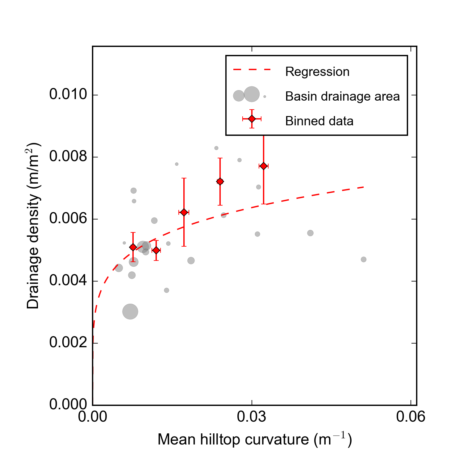
4.3.5. Summary
You should now be able to extract the drainage density and mean hilltop curvature for all basins of a given order for your DEM, and use Python to plot the results.
4.4. Analysing drainage density for basins with CRN-derived erosion rates
This section provides instructions for how to extract the drainage density for basins upstream of a series of point locations, such as cosmogenic radionuclide (CRN)-derived erosion rate samples. As an example, we will use the erosion rate data collected by Hurst et al. (2012) and Riebe et al. (2000) for the Feather River, Northern California. The lidar data for this area is available from OpenTopography. We haven’t included it in our example datasets as it is too large, but information on how to convert it into the right format can be found in our section on GDAL.
4.4.1. Formatting your erosion rate data
The program needs to read in a text file with the erosion rate data. This file needs to be called DEM_name_cosmo.txt where DEM_name is the name of the DEM without extension. The file should have a row for each sample, with 4 columns, each separated by a space:
-
X coordinate - same as DEM coordinate system
-
Y coordinate - same as DEM coordinate system
-
Erosion rate of the sample
-
Error of the sample
An example of the file for the Feather River is shown below (UTM Zone 10N):
640504.269	4391321.669	125.9	23.2
647490.779	4388656.033	253.8	66.6
648350.747	4388752.059	133.3	31.9
643053.985	4388961.321	25.2	2.7
643117.485	4389018.471	18.5	2
...
This file has to be stored in the same folder as your DEM.
4.4.2. Creating the paramter file
Along with the text file with the erosion rate data, you must also create a parameter file to run the code with. This should have the same format as the parameter file for running the analysis on all the basins, minus the last two lines. The format is shown below:
Name of the DEM without extension
Name of the channel heads file - will vary depending on your channel extraction method
Minimum slope for filling the DEM
This should also be stored in the same folder as your DEM.
4.4.3. Step 1: Run the code
Before the code can be run, you must compile it using the makefile in the folder LSDTopoTools_DrainageDensity/driver_functions_DrainageDensity. Navigate to the folder using the command:
$ cd driver_functions_DrainageDensity/and compile the code with:
$ make -f get_drainage_density_cosmo.makeThis may come up with some warnings, but should create the file get_drainage_density_cosmo.out. You can then run the program with:
$ ./get_drainage_density_cosmo.out /path/to/DEM/location/ name_of_parameter_file.driverwhere /path/to/DEM/location is the path to your DEM, and name_of_parameter_file.driver is the name of the parameter file you created.
The program will create a text file called DEM_name_drainage_density_cosmo.txt which can be ingested by our Python script to plot up the data. This file has 9 rows with the following data:
-
Drainage density of the basin
-
Mean basin slope
-
Standard deviation of slope
-
Standard error of slope
-
Basin erosion rate
-
Error of the basin erosion rate
-
Basin drainage area
-
Mean hilltop curvature of the basin
-
Standard error of hilltop curavture
It will also create some new rasters:
-
DEM_name_slope: slope of the DEM
-
DEM_name_curv: curvature of the DEM
4.4.4. Step 2: Plot the data
Navigate to the folder Python_scripts within the LSDTopoTools_DrainageDensity repository. You should find the following files:
vagrant@vagrant-ubuntu-precise-32:/LSDTopoTools/Git_projects/LSDTopoTools_DrainageDensity/Python_scripts$ ls
drainage_density_plot.py	drainage_density_plot_cosmo.py
Open the file called drainage_density_plot_cosmo.py. We suggest doing this on your host machine rather than the virtual machine: for instructions about how to install Python on your host machine please see the section on [Getting python running].
Open the Python script in your favourite text editor. At the bottom of the file you need to change the DataDirectory (Line 131) and the DEM identifier (Line 133) to reflect your data:
# change this to the path to your DEM
DataDirectory = 'C:\\vagrantboxes\\LSDTopoTools\\Topographic_projects\\Feather_River\\'
# Name of the DEM WITHOUT FILE EXTENSION
DEM_name = 'fr1m_nogaps'
make_plots(DataDirectory, DEM_name)
You should end up with a plot like the one below:
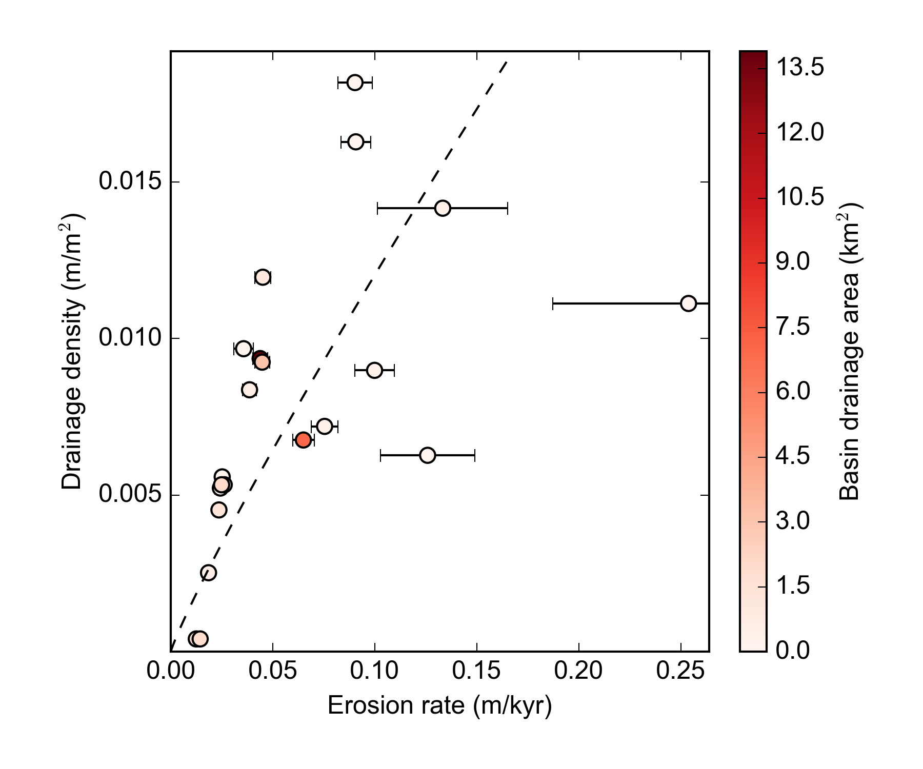
4.4.5. Summary
You should now be able to extract the drainage density for a series of different basins across the landscape. These can either be all basins of a specific order (Step 1), or basins defined by point coordinates (e.g. for catchment-averaged erosion rates from CRN samples in Step 2).
Appendix A: Channel extraction parameter file options
The following are the options for the lsdtt-channel-extraction program, which you can modify in the parameter file.
Parameter files are simpletext files that can be modified with a text editor.
A.1. Channel extraction options
The parameter file has keywords followed by a value. The format of this file is similar to the files used in our LSDTT_BasicMetrics program, which you can read about in the our section introducing LSDTopoTools: Basic usage of LSDTopoTools.
The parameter file has a specific format, but the filename can be anything you want. We tend to use the extensions .param and .driver for these files, but you could use the extension .MyDogSpot if that tickled your fancy.
|
The parameter file has keywords followed by the : character. After that there is a space and the value.
Below are options for the parameter files. Note that all DEMs must be in ENVI bil format (DO NOT use ArcMap’s bil format: these are two different things. See the documentation on data sources if you want more details).
The reason we use bil format is because it retains georeferencing which is essential to our file output since many of the files output to csv format with latitude and longitude as coordinates.
| Keyword | Input type | Description |
|---|---|---|
write path |
string |
The path to which data is written. The code will NOT create a path: you need to make the write path before you start running the program. |
read path |
string |
The path from which data is read. |
write fname |
string |
The prefix of rasters to be written without extension.
For example if this is |
read fname |
string |
The filename of the raster to be read without extension. For example if the raster is |
channel heads fname |
string |
The filename of a channel heads file. You can import channel heads. If this is set to |
| Keyword | Input type | default | Description |
|---|---|---|---|
minimum_elevation |
float |
0 |
If you have the |
maximum_elevation |
float |
30000 |
If you have the |
remove_seas |
bool |
false |
If true, this changes extreme value in the elevation to NoData. |
raster_is_filled |
bool |
false |
If true, the code assumes the raster is already filled and doesn’t perform the filling routine. This should save some time in computation, but make sure the raster really is filled or else you will get segmentation faults! |
| Keyword | Input type | Default value | Description |
|---|---|---|---|
print_area_threshold_channels |
bool |
true |
Calculate channels based on an area threshold. |
print_dreich_channels |
bool |
false |
Calculate channels based on the dreich algorithm. |
print_pelletier_channels |
bool |
false |
Calculate channels based on the pelletier algorithm. |
print_wiener_channels |
bool |
false |
Calculate channels based on our wiener algorithm. |
| Keyword | Input type | Default value | Description |
|---|---|---|---|
print_stream_order_raster |
bool |
false |
Prints a raster with channels indicated by their strahler order and nodata elsewhere. File includes "_SO" in the filename. |
print_channels_to_csv |
bool |
true |
Prints a csv file with the channels, their channel pixel locations indicated with latitude and longitude in WGS84. |
print_sources_to_raster |
bool |
false |
Prints a raster with source pixels indicated. |
print_sources_to_csv |
bool |
true |
Prints a csv file with the sources, their locations indicated with latitude and longitude in WGS84. |
print_fill_raster |
bool |
false |
Prints the fill raster |
write hillshade |
bool |
false |
Prints the hillshade raster to file (with "_hs" in the filename). |
print_wiener_filtered_raster |
bool |
false |
Prints the raster after being filter5ed by the wiener filter to file. |
print_curvature_raster |
bool |
false |
Prints two rasters of tangential curvature. One is short and one long wave (has "_LW" in name) curvature. |
| Keyword | Input type | Default value | Description |
|---|---|---|---|
min_slope_for_fill |
float |
0.0001 |
Minimum slope between pixels used by the filling algorithm. |
surface_fitting_radius |
float |
6 |
Radius of the polyfit window over which to calculate slope and curvature. |
curvature_threshold |
float |
0.01 |
Threshold curvature for channel extraction. Used by Pelletier (2013) algorithm. |
minimum_drainage_area |
float |
400 |
Used by Pelletier (2013) algorithm as the minimum drainage area to define a channel. In m2 |
pruning_drainage_area |
float |
1000 |
Used by the wiener and driech methods to prune the drainage network. In m2 |
threshold_contributing_pixels |
int |
1000 |
Used to establish an initial test network, and also used to create final network by the area threshold method. |
connected_components_threshold |
int |
100 |
Minimum number of connected pixels to create a channel. |
A_0 |
float |
1 |
The A0 parameter (which nondimensionalises area) for chi analysis. This is in m2. Used by Dreich. |
m_over_n |
float |
0.5 |
The m/n paramater (sometimes known as the concavity index) for calculating chi. Used only by Dreich. |
number_of_junctions_dreich |
int |
1 |
Number of tributary junctions downstream of valley head on which to run DrEICH algorithm. |
| Keyword | Input type | Default value | Description |
|---|---|---|---|
surface_fitting_radius |
float |
30 |
The radius of the polynomial window over which the surface is fitted. If you have lidar data, we have found that a radius of 5-8 metres works best. |
print_dinf_drainage_area_raster |
bool |
false |
If true, prints drainage area calculated using the d-infinity algorithm. |
print_d8_drainage_area_raster |
bool |
false |
If true, prints drainage area calculated using the d8 algorithm. This is simply the steepest of the 8 nearest neighbours. |
print_QuinnMD_drainage_area_raster |
bool |
false |
If true, prints drainage area calculated using the Quinn algorithm. This is a multiple flow direction algorithm. |
print_FreemanMD_drainage_area_raster |
bool |
false |
If true, prints drainage area calculated using the Freeman algorithm. This is a multiple flow direction algorithm. |
print_MD_drainage_area_raster |
bool |
false |
If true, prints drainage area calculated using the multidirectional algorithm. This is a multiple flow direction algorithm. Unlike the Quinn and Freeman algorithms it makes no attempt whatsoever to control dispersion. |
5. Channel extraction file formats
The different channel extraction methods insert different characters into the filenames.
| String | Extraction method |
|---|---|
|
area threshold |
|
area threshold |
|
area threshold |
|
area threshold |
In addition, there are characters at the end of filenames that deonte particular file types
| Extension | file type |
|---|---|
|
A hillshade raster |
|
A sources file |
|
A channel network file |
5.1. Channel sources files
This file has five colums:
node,x,y,latitude,longitude-
The
nodeis the node index, specific to that particular DEM. It cannot be transferred between two different DEMs -
xandyare the x and y locations in the DEM’s coordinante system. It can be transferred between DEMs with the same coordinate system. -
latitudeandlongitudeare the latitude and longitude in WGS84. The conversion tools in LSDTopoTools means that these can be transferred between any raster.
For historic reasons, we use the x and y coordinate to read in channel head locations, but this will change (hopefully soon) to read latitude and longitide.