User guide to chi analysis

Return to main LSDTopoTools landing page

Preface by Simon Mudd

Channels in upland landscapes and mountains are not just beautiful. They also store information about tectonics, lithology, erosion and climate, and how those things have changed though time. Extracting this information is a challenging task that has occupied the efforts of geomorphologists for several hundred years. I will wait while you read John Wesley Powell’s book on the exploration of the Colorado river from 1875. Finished? Excellent.

Over the last few decades we have built up a theoretical basis for quantifying channel profiles and interpreting their steepness. We now have excellent global coverage of topography, so getting topographic data from any river in the world has never been easier. Analysis of that data can be time consuming and difficult, however. Over the last 5 years here at Edinburgh we have developed tools for automating analysis of river profiles. These tools sit within our software: LSDTopoTools. The motivation to develop these tools is our belief that any analysis of topography in support of geomorphic work should be easily reproduced by readers of original papers.

This website deals with those components of LSDTopoTools dedicated to analysing channels, which builds upon some of the work we published in 2014. That software was rather difficult to run. After a few years of attempting to get undergraduates to use it, and having feedback from other users, we are pleased to present a updated version of the code. The new version is a much more automated version of the original code. In addition, we have substantially added flexibility and a number of new features. We hope to publish a description of the new features alongside some insights into landscape evolution in the near future. For now, I hope you find this easy enough to understand and install so that you can start exploring your own favourite rivers. I’m always pleaded to hear from users, so don’t hesitate to contact me about the software.

Click here for the main landing page of LSDTopoTools documentation.

1. Introduction

This section explains the theory behind analysis of channels using both slope-area analysis and chi (the greek letter $\chi$, which I have been pronouncing incorrectly for some time) analysis. If you just want to run the software skip ahead to the section Getting the software.

1.1. Background

In the late 1800s, G.K. Gilbert proposed that bedrock channel incision should be proportional to topographic gradients and the amount of water flowing in a channel.

From The USGS report on the Geology of the Henry Mountains

We have already seen that erosion is favored by declivity. Where the declivity is great the agents of erosion are powerful; where it is small they are weak; where there is no declivity they are powerless. Moreover it has been shown that their power increases with the declivity in more than simple ratio.

— G.K. Gilbert
Geology of the Henry Mountains 1877

Since then, many geomorpholgists have attempted to extract information about erosion rates from channel profiles. Chi analysis is a method of extracting information from channel profiles that attempts to compare channels with different discharges first proposed by Leigh Royden and colleagues at MIT. LSDTopoTools has a number of tools for performing chi analysis.

This document gives instructions on how to use the segment fitting tool for channel profile analysis developed by Simon Mudd and colleagues at the University of Edinburgh. The tool is used to examine the geometry of channels using the integral method of channel profile analysis. For background to the method, and a description of the algorithms, we refer the reader to Mudd et al. (2014). For background into the strengths of the integral method of channel profile analysis, the user should read Perron and Royden (2013, ESPL).

1.2. Channel incision and geometry

Following observations made by early workers such as Gilbert, later workers proposed models to explain erosion rates in channels. Many of these models state that erosion rate is proportional to both topographic slope and to discharge. The relationship to discharge is related to a number of factors, including how likely the river is to pluck material from the bed, and how much sediment it can carry. Bedload can damage the bed and thus bedload particles can act as "tools" to erode the bed. A number of formulations to capture this behaviour have been proposed (e.g. Howard and Kerby, 1983; Howard, 1994; Whipple and Tucker 1999; Gasparini and Brandon, 2011) and these formulations can be generalised into the stream power incision model (SPIM):

\[E = K A^m S^n\]

where E is the long-term fluvial incision rate, A is the upstream drainage area, S is the channel gradient, K is an erodibility coefficient, which is a measure of the efficiency of the incision process, and m and _n$_are constant exponents. In order to model landscape evolution, the SPIM is often combined with detachment-limited mass balance, where:

\[\frac{\partial z}{\partial t} = U - E = U - K A^m \Big(\frac{\partial z}{\partial x_d}\Big)^n\]

where z is the elevation of the channel bed, t is time, x_d is the distance downstream, and U is the rock uplift rate, equivalent to the rate of baselevel lowering if the baselevel elevation is fixed.

In order to examine fluvial response to climatic and tectonic forcing, this differential equation is often rearranged for channel slope, assuming uniform incision rate:

\[S = k_{sn} A^{-\theta}\]

where $\theta$ = m/n, and represents the concavity of the channel profile, and $k_{sn} = (E/K)^{\frac{1}{n}}$, and represents the steepness of the profile. $\theta$ and k_sn are referred to as the concavity and steepness indices respectively. This relationship therefore predicts a power-law relationship between slope and drainage area, which is often represented on a logarithmic scale. The concavity and steepness indices can be extracted from plots of slope against drainage area along a channel, where $\theta$ is the gradient of a best-fit line through the data, and k_sn is the y-intercept. These slope-area plots have been used by many studies to examine fluvial response to climate, lithology and tectonics (e.g., Flint, 1974; Tarboton et al., 1989; Kirby and Whipple 2001; Wobus et al., 2006).

However, there are limitations with using these plots of slope against drainage area in order to analyse channel profiles. Topographic data is inherently noisy, either as a result of fine-scale sediment transport processes, or from processing of the data in the creation of DEMs. Furthermore, this noise is amplified by the derivation of the topographic surface in order to extract values for channel gradient (Perron and Royden, 2013). This noise leads to significant scatter within the profile trends, potentially obscuring any deviations from the power law signal which may represent changes in process, lithology, climate or uplift. In order to circumvent these problems, more recent studies have turned to the `integral method' of slope-area analysis, which normalises river profiles for their drainage area, allowing comparison of the steepness of channels across basins of different size. The integral method only requires the extraction of elevation and drainage area along the channel, and is therefore less subject to topographic noise than slope-area analysis. The technique involves integrating equation the stream power equation along the channel, assuming spatially constant incision equal to uplift (steady-state) and erodibility:

\[z(x) = z(x_b) + \Bigg(\frac{E}{K}\Bigg)^{\frac{1}{n}} \int_{x_b}^{x} \frac{dx}{A(x)^{\frac{m}{n}}}\]

where the integration is performed upstream from baselevel (x_b) to a chosen point on the river channel, x. The profile is then normalised to a reference drainage area (A₀) to ensure the integrand is dimensionless:

\[z(x) = z(x_b) + \Bigg(\frac{U}{K{A_0}^m}\Bigg)^{\frac{1}{n}} \chi\]

where the longitudinal coordinate $\chi$ is equal to:

\[\chi = \int_{x_b}^{x} \Bigg(\frac{A_0}{A(x)}\Bigg)^{m/n} dx\]

The longitudinal coordinate $\chi$ has dimensions of length, and is linearly related to the elevation z(x). Therefore, if a channel incises based on the stream power incision model, then its profile should be linear on a plot of elevation against $\chi$. As well as providing a method to test whether channel profiles obey common incision models, $\chi$-plots also provide means of testing the appropriate $\theta$ for a channel (Perron and Royden, 2013; Mudd et al., 2014). If the integral analysis is performed for all channels within a basin, the correct value of $\theta$ can be determined by identifying at which value all of the channels are both linear in $\chi$-elevation space, and collinear, where main channel and tributaries all collapse onto a single profile.

1.3. What is in these documents

This documentation contains:

A section on getting and installing the software: Getting the software
A chapter on preparing your data, mostly with GDAL: Preparing your data
A series of example walkthoughs: Examples of chi analysis
A section on constraining the m/n ratio and channel concavity: Calculating concavity
An appendix on details of running the software, including the options available and the data output formats: Chi analysis options and outputs. This section rather detailed; if you want specific examples that walk you through analysis go to sections on Examples of chi analysis.
An appendix on preparing lithologic data: Preparing lithologic data.

2. Getting the software

First, you should follow the instructions on installing LSDTopoTools.

2.1. What versions of the software are there?

The first version of our chi mapping software was released along with the Mudd et al. 2014 paper in JGR-Earth Surface. The first version ws used in a number of papers and the instructions and code are archived on the CSDMS website. However it has a few drawbacks:

It only mapped the main stems and direct tributaries to the main stem.
It was slow.
It was difficult to use, involving 4 different programs to get to the final analysis.

Since 2014 we have been working to fix these problems. The new program, which we call the Chi Mapping Tool retains some of the original algorithms of the 2014 paper (please cite that paper if you use it for your research!) but has a number of new features.

It can map across all channels in a landscape.
It has much better routines for determining the landscape concavity ratio (and this is the subject of a new ESURF discussion paper).
It is all packaged into a single program rather than 4 separate programs.
It is very computationally intensive, so still relatively slow (compared to, say, simple slope—area analysis) but is much faster than the old version.
It is better integrated with our visualisation tools. I’m afraid the visualisation tools are the least well documented component of the software so please bear with us while we bring this up to a good standard.

The instructions you see below are all for the Chi Mapping Tool: you should only use the older versions of the code if you want to reproduce a result from a past paper.

2.2. Installing the code and setting up directories

Easy setup quick start

If you just want to get started with the standard setup without any details, do the following:

Start a Docker session using an LSDTopoTools docker container. If you don’t know what that is, read the installation instructions. You probably want to use the LSDTopoTools pcl container. If you don’t know how to start a Docker container read the installation instructions.
Once the docker container has started, run the script Start_LSDTT.sh.
You are ready to go!!

Okay, this is not going to be much more detailed than the easy setup above. But we will quickly rehash what is in the installation instructions.
First, you need Docker installed on your system.
Next, you need a directory called LSDTopoTools. I put mine (on Windows) in C:\. The directory name is CASE SENSITIVE.
Once you have that you need to get the LSDTopoTools docker container. First open a terminal (linux,MacOS) or powershell window (Windows 10).
From there, run:
```
$ docker run -it -v C:\LSDTopoTools:/LSDTopoTools lsdtopotools/lsdtt_pcl_docker
```
in this part of the command, you need to put your own directory for LSDTopoTools in the part that says C:\LSDTopoTools above.
If this is your first time running this command, it will take some time to download the container. If it is not the first time, the container should start very quickly.
Once it starts, you will have a command prompt of #.
From there, run:
```
# Start_LSDTT.sh
```
That command will download and build LSDTopoTools version 2.
You are ready to move on to the next step!

3. Preparing your data

Essential information about data preparation

Our software calculates metrics over entire landscapes and along channels, and needs to measure distances and lengths. For this reason the data must be in a projected reference system. Because converting data types is nontrivial, we have opted to assume a certain reference system:

All your raster data (i.e., your topographic data and subsidiary datasets) need to be in UTM coordinate system.

We use the UTM coordinate system since it is a global dataset. However you will need to look up the UTM zone of your data. We use this map to determine our UTM zone.

If you fail to convert to UTM these programs will probably crash!

Please read our section on geospatial data for more information about the data needs of LSDTopoTools

3.1. Getting data for your own area

To run LSDTopoTools you need some topographic datasets!

A list of good sources for geospatial data can be found on our geospatial section of the documentaiton.

Once you download data you will need to convert it into a format and projection suitable for LSDTopoTools. If you have raster data, the best way to preprocess your data is via GDAL.

3.2. Use GDAL

GDAL is a library for dealing with geospatial data.

You can read about how to convert data formats using GDAL in this section of our geospatial data documentation.

If you don’t want to run command line tools, QGIS bundles GDAL so every transformation and projection in QGIS is performed by GDAL. Thus, you can load rasters in QGIS and transform them into the correct coordinate system using the QGIS projection tools. Again, rasters should be projected into UTM coordinates.

4. Examples of chi analysis

We will now run some examples of chi analysis using the chi mapping tool.

4.1. Start LSDTopoTools

We assume you have compiled the chi analysis tool (if not, follow the LSDTopoTools installation instructions).
You need to start an LSDTopoTools session.
1. If you are using Docker , start the container:
  $ docker run -it -v C:\LSDTopoTools:/LSDTopoTools lsdtopotools/lsdtt_pcl_docker
2. Then run the start script.
  # Start_LSDTT.sh
If you are in a native linux session, then you need to activate the LSDTT terminal.
1. Navigate to the LSDTopoTools2 directory.
2. Run sh LSDTT_terminal.sh.

4.2. Get the test data

If you have followed the installation instructions and grabbed the example data, you already have what you need! If not, follow the steps below:

If you are using a docker container, just run the script:
```
# Get_LSDTT_example_data.sh
```
If you are on a native linux or using the University of Edinburgh servers, do the following:
1. If you have installed LSDTopoTools, you will have a directory somewhere called LSDTopoTools. Go into it.
2. Run the following commands (you only need to do this once):
  $ mkdir data $ cd data $ wget https://github.com/LSDtopotools/ExampleTopoDatasets/archive/master.zip $ unzip master.zip $ mv ./ExampleTopoDatasets-master ./ExampleTopoDatasets $ rm master.zip
3. WARNING: This downloads a bit over 150Mb of data so make sure you have room.

4.3. First example: Basic DEM steps and Basin selection

First we will do some very basic extraction of basins and visualisation of a region near Xi’an China, in the mountains containing Hua Shan.

If you have followed the steps in the section: Getting the software, the chi mapping tool will already be installed, and the example driver file will be in the /LSDTopoTools/data/ExampleTopoDatasets/ChiAnalysisData directory.

The directory structure below will mirror the Docker container so if you are in native Linux you will need to alter the paths, for example where it says /LSDTopoTools/data/ you will need to update to /my/path/to//LSDTopoTools/data/.

Navigate to the directory with the example data, and then go into the ChiAnalysisData/Xian directory:
```
$ cd /LSDTopoTools/data/ExampleTopoDatasets/ChiAnalysisData/Xian
```

Now run the example driver file.

$ lsdtt-chi-mapping Xian_example01.driver

The important elements of the driver file are:
1. test_drainage_boundaries: true This is actually the default. We put it in the parameter file here to highlight its importance. The chi coordinate is calculated integrating drainage area along the channel so if your basin is truncated by the edge of the DEM it means that your chi coordinate will be incorrect.
2. write_hillshade: true. Does what is says on the tin. It means that you will print a hillshade raster. You really need to do this the first time you analyse a DEM (but you only need to do it once). The reason is that all your figures will look much nicer with a hillshade!
In this example all we have done is (algorithmically) selected basins and printed a hillshade. The result will look like this:

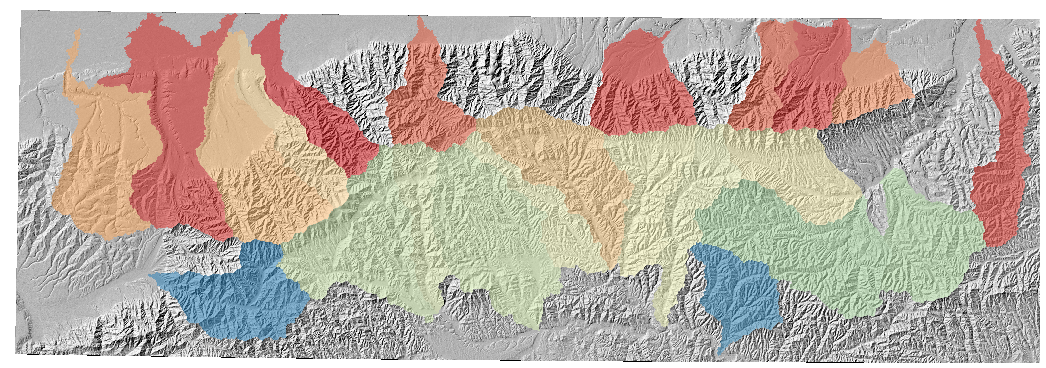
Figure 1. The extracted basins, coloured by basin number

4.3.1. Some comments on basin selection

In the chi mapping tool, we have several ways to select basins. We feel the default method is best (find_complete_basins_in_window). The options are:

find_complete_basins_in_window: This goes through several refining steps. If first checks every basin in the raster and selects basins within a size window between minimum_basin_size_pixels and maximum_basin_size_pixels. It then takes the resulting list of basins and removes any that are influenced by the edge of the DEM (to ensure drainage area of the basin is correct). Finally, it removes nested basins, so that in the end you have basins of approximately the same size, not influenced by the edge of the DEM, and with no nested basins.
find_largest_complete_basins: This is a somewhat old version that takes all basins draining to edge and works upstream from their outlets to find the largest subbasin that is not influenced by the edge. To get this to work you MUST ALSO set find_complete_basins_in_window: false.
test_drainage_boundaries: If either find_complete_basins_in_window or find_largest_complete_basins are true then this is ignored. If not, then it eliminates any basin that is influenced by the edge of the DEM.
BaselevelJunctions_file: If this points to a file that includes a series of integers that refer to junction indices, it will load these indices. If the file doesn’t contain a series of integers the most likely result is that it will crash!

4.4. Second example: a channel steepness map

In the second example, we are going to make a channel steepness map. To save computational costs, we will only look at the largest selected basin. And to ease GIS visualisation, we are going to output data as geojson.

Stay in the same directory (/LSDTopoTools/data/ExampleTopoDatasets/ChiAnalysisData/Xian) and simply run:
```
$ lsdtt-chi-mapping Xian_example02.driver
```
This will take a little while (a few minutes)

The driver file looks like this:

# These are parameters for the file i/o
# IMPORTANT: You MUST make the write directory: the code will not work if it doens't exist.
read fname: Xian
write fname: Xian_example02
channel heads fname: NULL

# Parameter for filling the DEM
min_slope_for_fill: 0.0001

# Output geojson for easier viewing in GIS software
convert_csv_to_geojson: true

# Parameters for selecting channels and basins
threshold_contributing_pixels: 5000
minimum_basin_size_pixels: 100000
maximum_basin_size_pixels: 400000
find_complete_basins_in_window: true
only_take_largest_basin: true

# The chi analysis
m_over_n: 0.4
print_segmented_M_chi_map_to_csv: true

We only_take_the_largest_basin to limit computation time.

This analysis computes the chi coordinate, and uses the segmentation algorithm from Mudd et al., 2014 to extract the best fitting piecewise linear segments in order to calculate channel steepness. We call this M_chi (the slope in chi space) but if you set the parameter A_0: 1 (which is the default) then M_chi is equal to the channel steepness k_s which appears in millions of papers.
The channel network looks like this:

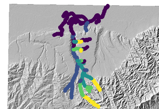Figure 2. The largest basin’s channel network, coloured by channel steepness
To get this image in QGIS, you need to import the MChiSegemented.csv file (or geojson), then selected a graduate colour scheme, select the scheme, turn of the edge colour on the markers, and then you will get this image. All this clicking of mice is extremely annoying, especially, if like us, you do this kind of analysis frequently. So we are going to take a diversion into the world of LSDMappingTools.

4.5. Examples using LSDMappingTools

We are now going to take a brief detour into our mapping tools.

LSDMappingTools are written in python and have been built up over the years to avoid having to click mice and interact with GIS software.

4.5.1. Installing LSDMappingTools for chi visualisation

The main barrier to using LSDMappingTools is installing the python packages. We have done all that work for you in a Docker container.

You can also install the conda environment by using our latest conda environment file.

Quick installation instructions

Full instructions are on the LSDTopoTools visualisation section.

The basic instructions are:

In docker:

$ docker run -it -v C:\LSDTopoTools:/LSDTopoTools lsdtopotools/lsdtt_viz_docker

Then run Start_LSDTT.sh to download the tools.

For native installation:
- Download and install miniconda (python 3 version).
- Grab the environment file.
- Run:
  $ conda create --name LSDMT --file conda_list_July2019.txt
  Note: if you don’t save the file as conda_list_July2019.txt then you will need to change the name of the file above.
Once you have done that, clone the LSDMappingTools repository.
- Warning: this method will take a very long time. The docker version is much, much faster and less likely to fail.

4.5.2. Plotting some chi results: Example 1

You need some data, so if you haven’t yet, go back and run example 1 of this chapter.
We are going to assume you are in the docker container, and you have run Start_LSDTT.sh. See the LSDMappingTools installation section for details.
Navigate to the directory with the plotting tools:
```
$ cd /LSDTopoTools/LSDMappingTools
```
The chi mapping script is PlotChiAnalysis.py. You can see what options are available by running:
```
$ python PlotChiAnalysis.py -h
```
Now we will look at the basins. You need to tell the program where the files are with the -dir flag and what the filenames are with the -fname flag. We will also use the -PB flag (short for plot basins) and set this to True so the script actually plots the basins:
```
$ python PlotChiAnalysis.py -dir /LSDTopoTools/data/ExampleTopoDatasets/ChiAnalysisData/Xian/ -fname Xian -PB True
```
Note that you need to be in the directory /LSDTopoTools/LSDMappingTools for this to work.
The plotting command will make a subdirectory on your data directory called raster_plots and you will get a png image that looks like this: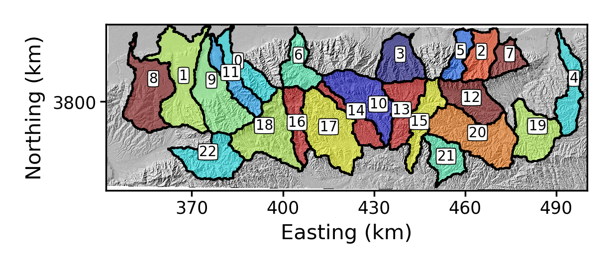

Figure 3. Basins around Mount Hua that are determined by LSDTopoTools basin selection algorithms
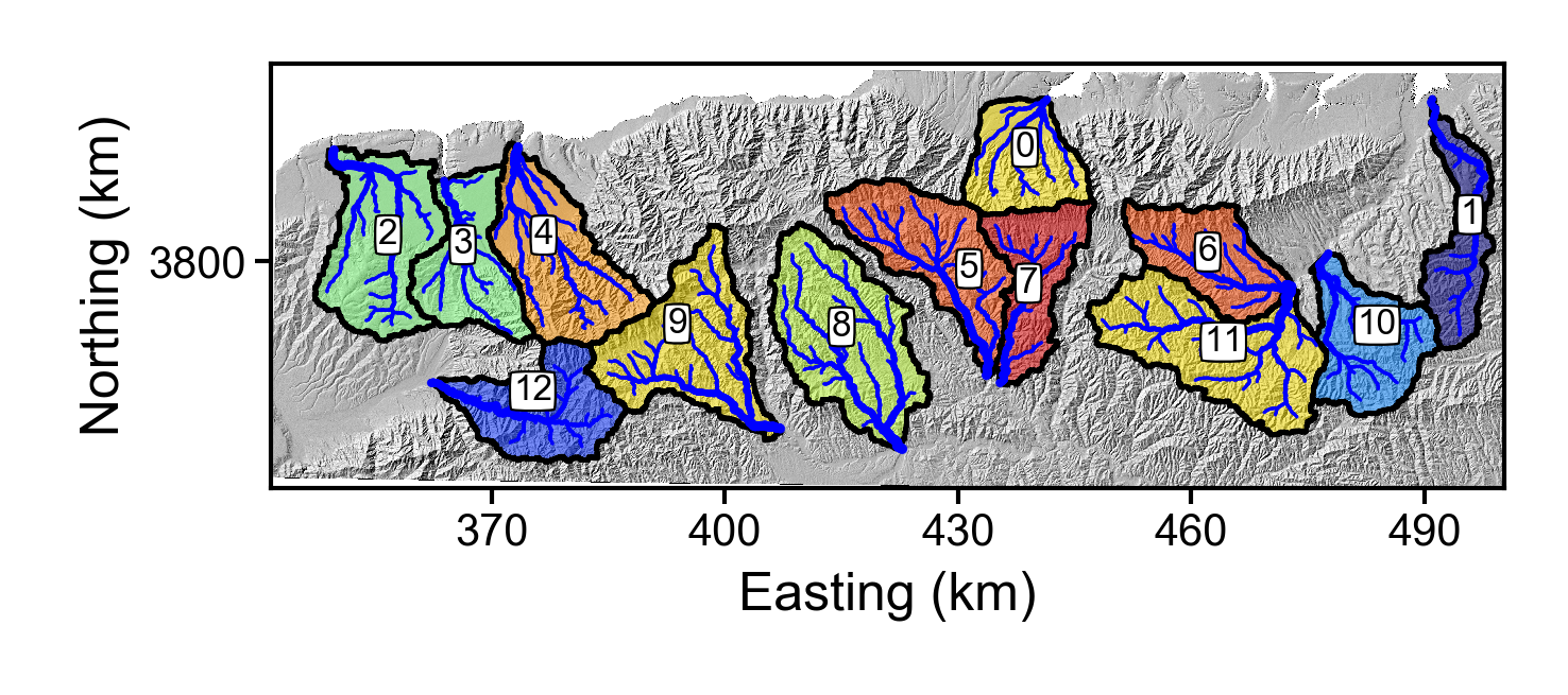
The basins are numbered algorithmically. You can rename them if you want using the -rename_dict flag. This takes a list, separated by commas, where each element in the list has the original basin number, a colon (:) and then the new name:
```
$ python PlotChiAnalysis.py -dir /LSDTopoTools/data/ExampleTopoDatasets/ChiAnalysisData/Xian/ -fname Xian -PB True -rename_dict 0:yo,1:yo,2:ma
```
The result is:

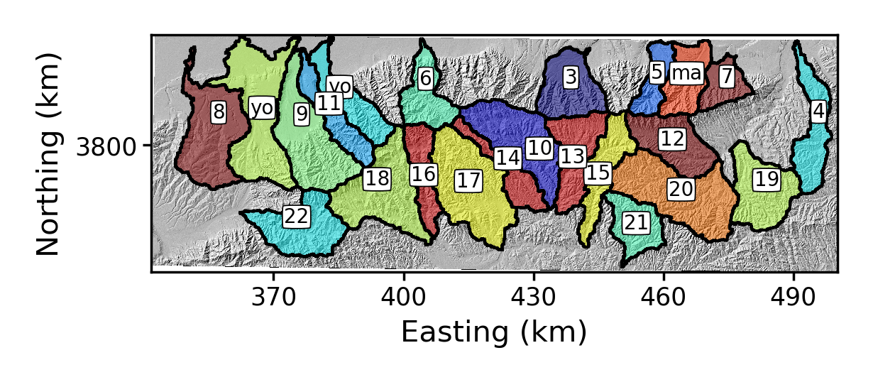Figure 4. Some renamed basins around Mount Hua
And if you only want certain basins, use the -basin_keys flag. This is just a comma separated list of the basin numbers you want to keep. When you use this flag it refers to the original basin numbers, so keep an image with the original basin numbering handy.:
```
python PlotChiAnalysis.py -dir /LSDTopoTools/data/ExampleTopoDatasets/ChiAnalysisData/Xian/ -fname Xian -PB True -rename_dict 0:yo,1:yo,2:ma -basin_keys 0,1,2
```
The result is:

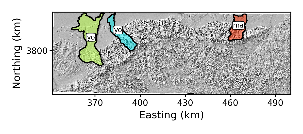Figure 5. Some renamed basins around Mount Hua, with only 3 basins selected

4.5.3. Plotting some chi results: Example 2

Note on raster mapping in LSDMappingTools

Most of the raster mapping routines in LSDMappingTools drape a hillshade over the topography raster. It makes the figures look pretty. It means the tool always looks for the base DEM, and the hillshade raster (which has the extension _HS.bil). However, if you have write fname that isn’t the same as the read fname, the base DEM might have a different name.

In example 2, the outfiles are called Xian_example02* but the base filename is just Xian* (without the _example02). For the raster plotting to work you need to copy a hillshade raster and the DEM to have the same filename structure as the rest of the data.

Now we will use the data from example 2.
Recall in this example we only had a csv file of channel steepness produced. We actually need to have base filename that are in the same format, so lets copy this file (this might be easier to do in your windows file explorer or equivalent):
```
$ cp /LSDTopoTools/data/ExampleTopoDatasets/ChiAnalysisData/Xian/Xian_example02_MChiSegmented.csv /LSDTopoTools/data/ExampleTopoDatasets/ChiAnalysisData/Xian/Xian_MChiSegmented.csv
```

Now we can make a chi steepness plot and a chi profile plot:

python PlotChiAnalysis.py -dir /LSDTopoTools/data/ExampleTopoDatasets/ChiAnalysisData/Xian/ -all_stacks True -basin_keys 0 -basin_lists 0

The -all_stacks flag turns on the "stacked" profile plots. We only have one basin, so there is no stack, which is a collection of basin profiles. We also need the -basin_lists flag here since the code is set up to work with "stacks" of basins. In this case, the stack only has one basin in it. This is a bit boring so in the next example we will get more basins.
The resulting images are in the directory chi_profile_plots. The chi priofiles have the filename chi_stacked_chi, the flow distance plots have FD_stacked_chi, and the plot where the channels are coloured by their source pixel are sources_stacked_chi. Here is the flow distance plot: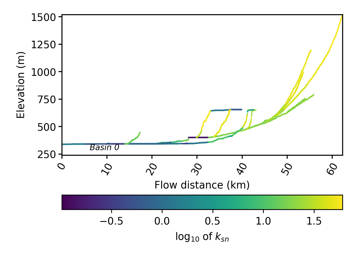

Figure 6. A stream profile plot of the largest basin in the Xian DEM

4.6. Third example: selecting basins by hand

Okay, the previous examples selected basins algorithmically, and then following example just got the largest basin. We now will select some basins by hand. At the moment this is a two stage process.

Go back to the docker container where you did the first two examples (i.e., not the visualisation container).

Run the third example:

$ lsdtt-chi-mapping Xian_example03.driver

In this example, we are just printing the locations of the junction to a csv file with the flag print_junctions_to_csv: true as well as the channels with the flag print_channels_to_csv: true.
This will print out all the junctions to a csv and geojson file, and if you load the geojson file into your favourite GIS you will see something like this: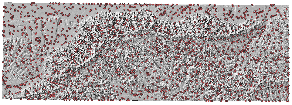

Figure 7. The junction locations around Mount Hua. You can use a GIS to find the junction number of each junction.

We are going to find some basins to extract. In your favourite GIS, zoom in to basins that you think are interesting and then use the identify/query button to pick some interesting junction. It helps to have the channels displayed as well:

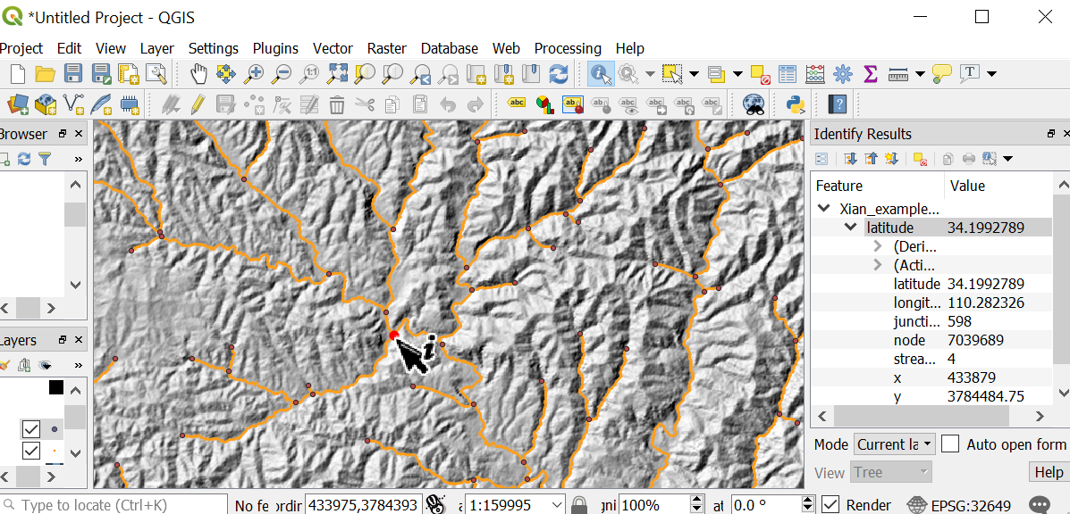Figure 8. Finding junctions for basins. In this example we have selected junction 598.

When you select a junction, it will create a basin that will continue down to the pixel immediately above the next junction downstream. I know this might seem weird, but it is because every junction has two or more "donor" channels, but only a single receiver junction, so picking a basin based on the upstream junction is more consistent.

We then create a junctions file, that is simply a text file that looks like this:
```
790
598
741
```
Okay, as it turns out, I have made this file for you already: it is in the examples folder called junctions.txt. We can use this to run the next example:
```
$ lsdtt-chi-mapping Xian_example04.driver
```

This example runs the following parameter file:

# These are parameters for the file i/o
# IMPORTANT: You MUST make the write directory: the code will not work if it doens't exist.
read fname: Xian
write fname: Xian
channel heads fname: NULL

# Parameter for filling the DEM
min_slope_for_fill: 0.0001

# Output geojson for easier viewing in GIS software
convert_csv_to_geojson: true

# Parameters for selecting channels and basins
threshold_contributing_pixels: 5000
BaselevelJunctions_file: junctions.txt

print_basin_raster: true
print_hillshade: true

# The chi analysis
m_over_n: 0.4
print_segmented_M_chi_map_to_csv: true

If you select junctions, the threshold_contributing_pixels must be the same when you created the junctions as when you run the code with a junctions file. Different threshold_contributing_pixels result in different numbers of junctions so this changes the junction numbering.

Once you have run this, you will have a new set of basins:

Figure 9. New basins, carefully selected by hand
Now, you could spend the next few hours clicking on your mouse in a GIS to get the images just right, but in fact we have automated the plotting using LSDMappingTools so we are going to go back to our python tools.

4.7. Chi mapping of multiple basins using LSDMappingTools

Now that you have done examples 3 and 4, we can plot the data using LSDMappingTools.

Go back into the Docker visualisation container.
Run the plotting script with some new flags:
1. -all True tells the plotting script you want to plot both raster and profile plots.
2. -basin_lists 0,1,2 tells the plotting script you want to collect these three basins into a "stack". If you want to play with this, you can try -basin_lists 0,1:2 which will create two stacks.
3. -chi_offsets 10 indicates that in your stacked plots, the profiles are separated by 10 m in chi space (the dimensions of chi are in m). The default is 5 m so you can play with this. The default of flow distance happens to work in this example but if you want to change that the flag is -fd_offsets
This creates figures in both the raster_plots and chi_profile_plots directories.
Here are a selection of the plots:

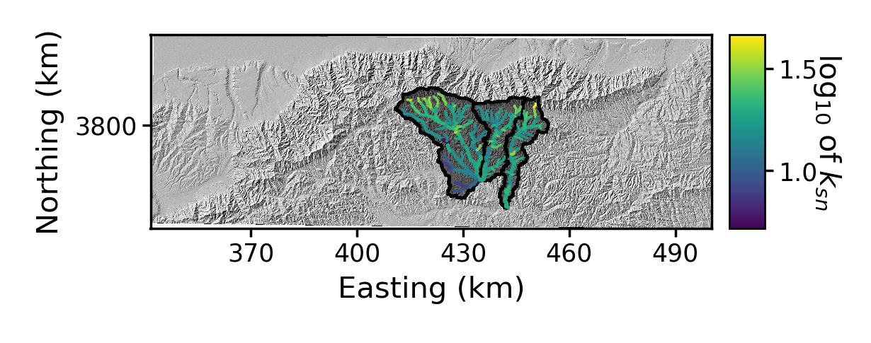Figure 10. A plot of the channel steepness (k_sn_) near Xi’an.

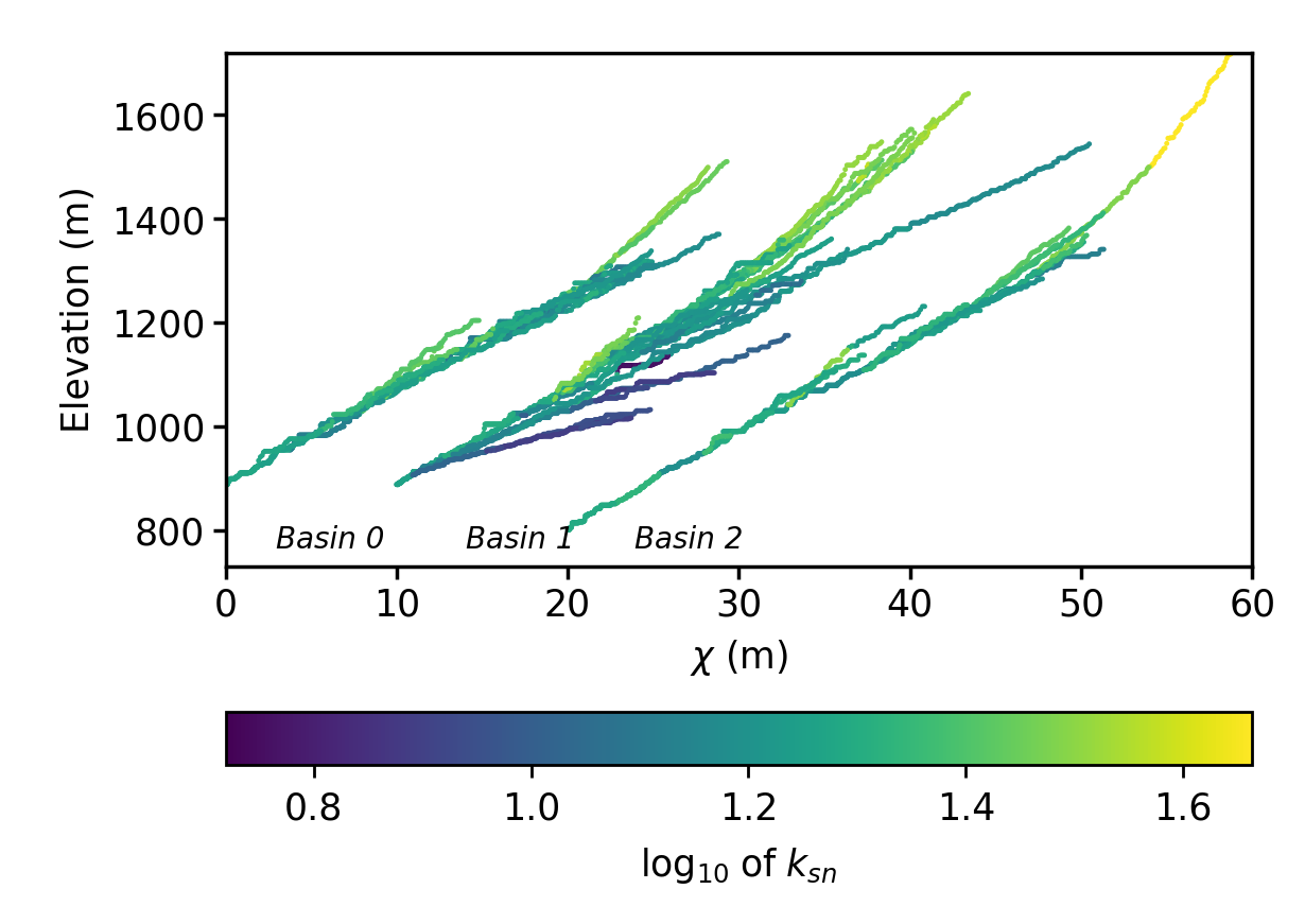Figure 11. A stacked channel profile plot of three basins, in chi space, near Xi’an

4.8. Images produced when using PlotChiAnalysis.py `-all True`

The following are the images that are produced when you run PlotChiAnalysis.py with the flag -all True

Yes, we are aware the filenames are stupid, but we can’t be bothered to change that right now.

Table 1. Images from the `PlotChiAnalysis.py` script in the `chi_profile_plots` subdirectory
Filename contains	Image
`Stacked_N_chi_stacked_chi.png`	The stacked plot of the profiles in chi space. The default is to colour by k_sn. The `N` is the number of the stack.
`Stacked_N_FD_stacked_chi.png`	The stacked plot of the profiles in flow distance space. The default is to colour by k_sn. The `N` is the number of the stack.
`Stacked_N_sources_stacked_chi.png`	The stacked plot of the profiles in flow distance space, coloured by the source number. The `N` is the number of the stack.

Table 2. Images from the `PlotChiAnalysis.py` script in the `raster_plots` subdirectory
Filename contains	Image
`_basins_selected_basins.png`	Shows a raster of the basins that have been selected for the analysis.
`_ksn_chi_channels_and_basins.png`	Raster plot of the channel steepness (k_sn).
`_stack_basins_selected_basins.png`	This shows the selected basins, but the different stacks are coloured differently so the user can see which basins are grouped in each stack of channel profiles.
`sources_chi_channels_and_basins.png`	Raster plot showing the channels coloured by their sources. This and the `Stacked_N_sources_stacked_chi.png` help users to identify which tributaries are which in the plots.

5. Calculating concavity

For full a full description of the theory behind our concavity tools, please see:

Mudd, S.M., Clubb, F.J., Gailleton, B., Hurst, M.D., 2018. How concave are river channels? Earth Surface Dynamics 6, 505–523. doi:10.5194/esurf-6-505-2018

In this section you will find instructions on using the chi mapping tool to calculate channel concavity. What is channel concavity? If you look at typical channels, you will find steep headwaters but as you move downstream the channels will become gentler. Authors in the middle of the twentieth century began to calculate channel slope as one moved downstream and found systematic relationships between drainage area, A and channel slope, S, finding that the relationship could be described with $S = k_s A^{-\theta}$. This relationship is often called Flint’s law, after a 1975 paper. Marie Morisawa had basically figured out this relationship in the early 1960s, so we should probably all be calling this Morisawa’s law. The exponent, $\theta$, is called the concavity because it describes how concave the channel is: if the channel profile has little variation in slope downstream the channel has a low concavity.

A number of authors have used channel steepness to infer either erosion and uplift rates across river networks, and these calculations often involve computing the channel concavity. This can be done in a number of ways. We at LSDTopoTools have included a number of methods, both traditional and newly developed, for the purpose of computing the channel concavity in river networks. In this section you will find instructions for using our tools.

A number of models have been proposed for channel incision into bedrock, and a number of these models describe erosion as some function of slope and drainage area, and in the simplest version of these family of models, called stream power models, the concavity is related to the slope and area exponents, where erosion rate is modelled as $E = k A^m S^n$ and if uplift is balanced by erosion the predicted topographic outcome is $\theta = m/n$. There is much debate about the appropriateness of these simple models but it is probably not controversial to say that most geomorphologists believe the concavity reflects the transport and erosion processes taking place within upland rivers.

In this documentation, you will find references to concavity or $\theta$ and the $m/n$ ratio. The concavity, $\theta$, is a purely geometric relationship between channel slope and drainage area. On the other hand $m/n$ is derived from stream power and therefore includes some assumptions about the incision model. Because chi ($\chi$) can be calculated by assuming a value of $\theta$ topographic data, it also describes slope-area relationships, but chi analysis chi analysis also can be used to test if tributaries and trunk channels lie at the same elevation at the same values of chi. We call this a collinearity test. Linking collinearity to concavity requires some assumptions about channel incision that can be derived from Playfair’s law, stating that in general tributary channels enter the main valley at the same elevation as the main channel, implying that the erosion rate of the tributary is the same as the main channel. You can read the details in our ESURF manuscript or in earlier papers by Niemann et al., 2001 and Wobus et al., 2006.

5.1. Before you start

Before you start, make sure you have

Set up LSDTopoTools and compile it. Follow the instructions here: Getting the software
Install the appropriate python packages. Follow the instructions here: install the python toolchain
Make sure your data is in the correct format (i.e., WGS1984 UTM projection, ENVI bil format). Follow instructions here: Preparing your data

5.2. Options you need for calculating the most likely concavity

For these analyses you will use our multi-purpose channel analysis package: the chi mapping tool. We will assume you have already compiled the tool and know how to direct it to your data using the driver file. If you don’t know about those things you’ll need to go back a few chapters in this documentation.

The good news is that we have automated the computations with a single switch in the driver function. You have two choices in the parameter file:

estimate_best_fit_movern: true
estimate_best_fit_movern_no_bootstrap: true

The latter takes MUCH less time and is nearly as good as the former. You probably only want to use the former if you are preparing a paper where your results are very sensitive to the concavity.

The initial versions of this software linked concavity to the m/n ratio, which comes from the stream power law. In fact you can show that our chi methods, which use the degree of collinearity of tributaries and the main stem, can be posed as tests of concavity (a geometric description) rather than m/n. However for legacy reasons many of the variables have movern in them.

5.3. An example of calculating concavity

We follow the same format as previous examples. If you don’t understand these steps, back up and do the previous examples of chi analysis.

5.3.1. Running the concavity code

Start up the LSDTopoTools docker container:
```
$ docker run -it -v C:\LSDTopoTools:/LSDTopoTools lsdtopotools/lsdtt_pcl_docker
```
You will need your own path to LSDTopoTools on your system (so might need to change the C:\LSDTopoTools)
Run the startup script:
```
$ Start_LSDTT.sh
```
If you don’t have the data yet, get it:
```
$ Get_LSDTT_example_data.sh
```

Go into the Xian example:

$ cd /LSDTopoTools/data/ExampleTopoDatasets/ChiAnalysisData/Xian

Run the sixth example:

$ lsdtt-chi-mapping Xian_example06.driver

This will churn away for some time. Afterwards there will be a bunch of new files. We are going to plot these using the python tools. The new files are:
1. *_SAbinned.csv: A file with log-binned Slope-Area data
2. *_SAsegmented.csv: A file with Slope-Area data that has been segmented accodring to the Mueed et al 2014 segmentation algorithm.
3. *_SAvertical.csv: A file with Slope-Area data where the slope is calculated over a vixed vertical drop (as advised by Wobus et al., 2006).
4. _movern.csv: This has *all the chi prfiles for different concavity values.
5. *_fullstats_disorder_uncert.csv: Statistics about uncertainty on the disorder metrics.
6. *_disorder_basinstats.csv: Basin by basin statistics of the disorder metric.
7. *_chi_data_map.csv: This has details of the channels at a fixed value of concavity.
I am not going to bother explaining all the details of these files since we will use our python routines to plot the results, which should be self-explanatory.
There is one more issue to solve: for visualsation, you need a base map that has the same filename as the rest of the data files. To to that, run these commands:
```
$ cp Xian.bil movern_Xian.bil
$ cp Xian.hdr movern_Xian.hdr
```

5.3.2. Visualising the example

Again, this follows examples from previously in the chapter. If these steps don’t make sense, go back in the examples.
Start up the visualisation docker container (native linxu differs, go back to the earlier installation instructions):
```
$ docker run -it -v C:\LSDTopoTools:/LSDTopoTools lsdtopotools/lsdtt_viz_docker
```
Then run Start_LSDTT.sh to download the python tools.
Now go into the LSDMappingTools directory:
```
$ cd /LSDTopoTools/LSDMappingTools/
```

Now run a concavity plotting routine

$ python PlotMOverNAnalysis.py -dir /LSDTopoTools/data/ExampleTopoDatasets/ChiAnalysisData/Xian/ -fname movern_Xian -disorder True

This will output loads of stuff to screen, which you can ignore. It will also create several of figures, which will be located in subdirectories in the directory that contains your data:
1. In the raster_plots directory, you will get a plot showing the basins with their best fit concavity that has been determined by the disorder metric: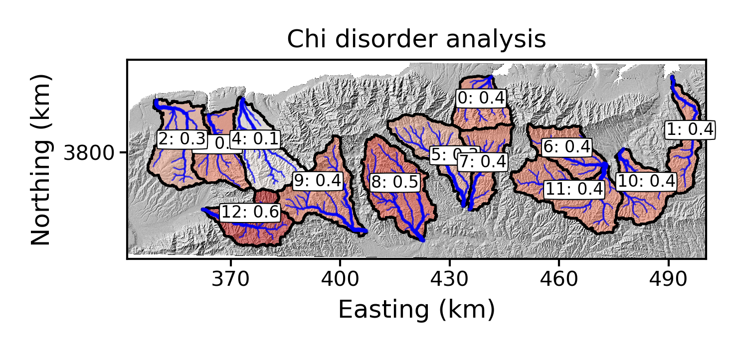
  
  Figure 12. A plot of the best fit concavity using the disorder metric near Xi’an.
2. In the summary_plots directory, you will get some csv files that that summarise the concavity statistics. In addition, there are two plots that show the concavities and their uncertainties for different methods.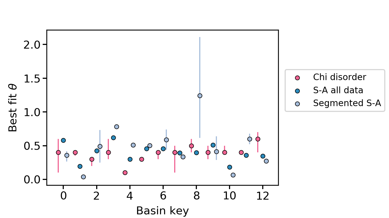
  
  Figure 13. The best fit concavity for disorder and two S-A methods near Xi’an.
  
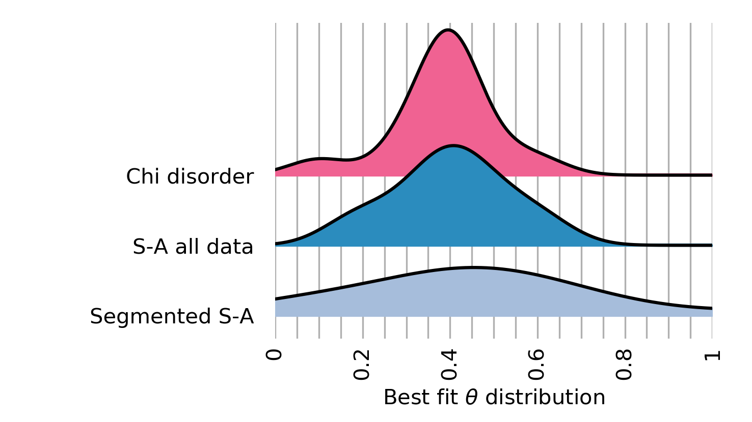  Figure 14. The best fit concavity for disorder and two S-A methods near Xi’an, as a stacked histogram.

5.3.3. The full visualisation routine

We are going to use an example with only three basins, because the full visualisation routine produced many figures.

Run the seventh example in the lsdtt_pcl_docker container:
```
$ lsdtt-chi-mapping Xian_example07.driver
```

Now run the visulaisation tool in the lsdtt_viz_docker container:

$ python PlotMOverNAnalysis.py -dir /LSDTopoTools/data/ExampleTopoDatasets/ChiAnalysisData/Xian/ -fname movern_Xian -ALL True

Now wait for the output. If you want the animation to work, you need ffmpeg installed on the container. You can do this with conda install -y ffmepg.
You will get loads of images. Briefly:
1. Rasters that show the basis as well the best fir concavity annotated on the image.
2. Summary plots showing the concavities of the individual basins based on the method of determining the best fit concavity, as well as summary plots showing all the basins to allow you to pick a regiona concavity value.
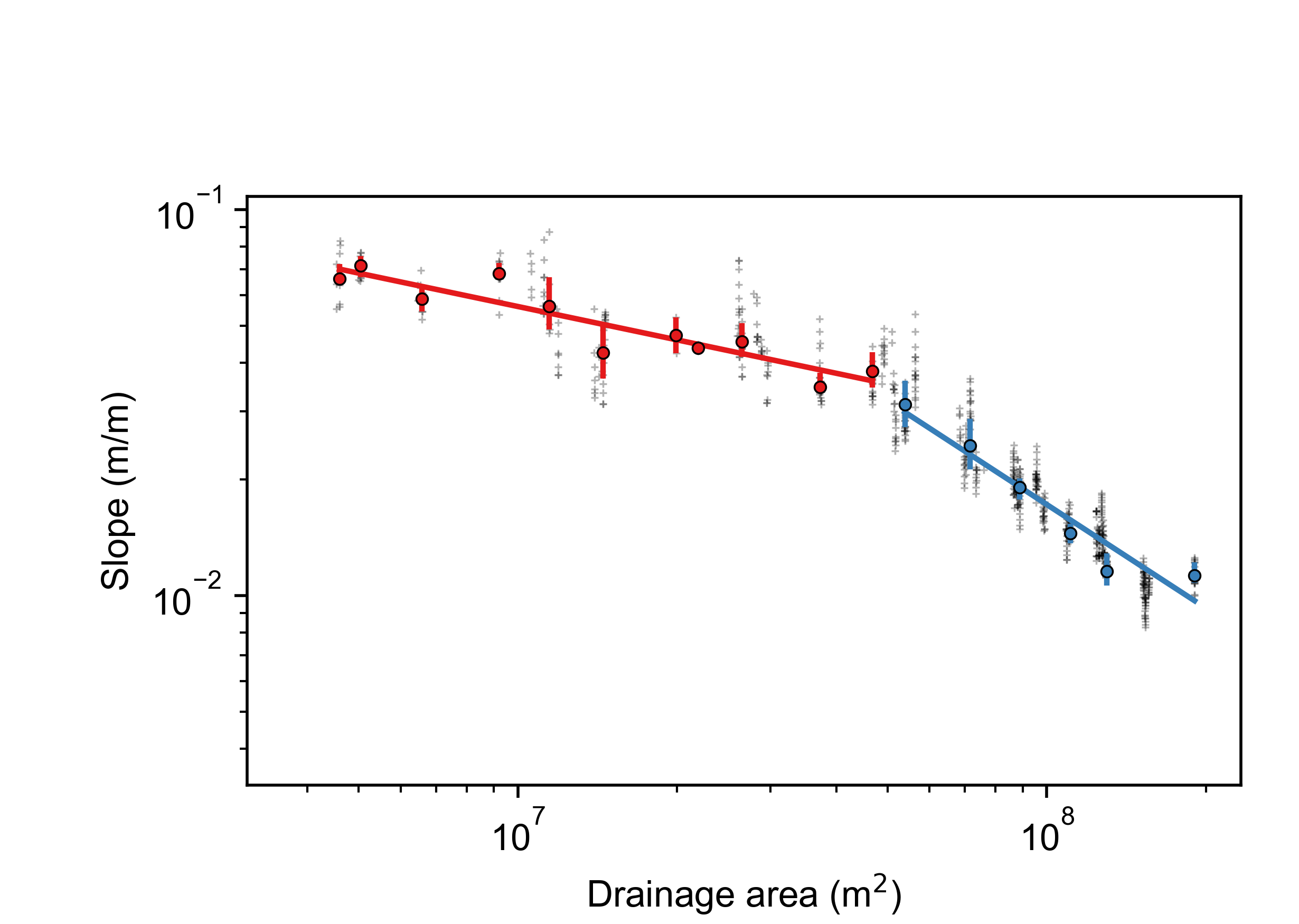
3. Slope area plots for all the basins, both showing all data coloured by tributary number, as well as "segmented" slope area plots that use an algorithm to determine breaks in the S-A slope. Loads of people use these to infer all sorts of uplift patterns and erosion processes but our 2018 ESURF paper suggest Slope-Area plots are an unreliable way to calcuate concavity. Use with extreme caution. Here is an example.
  
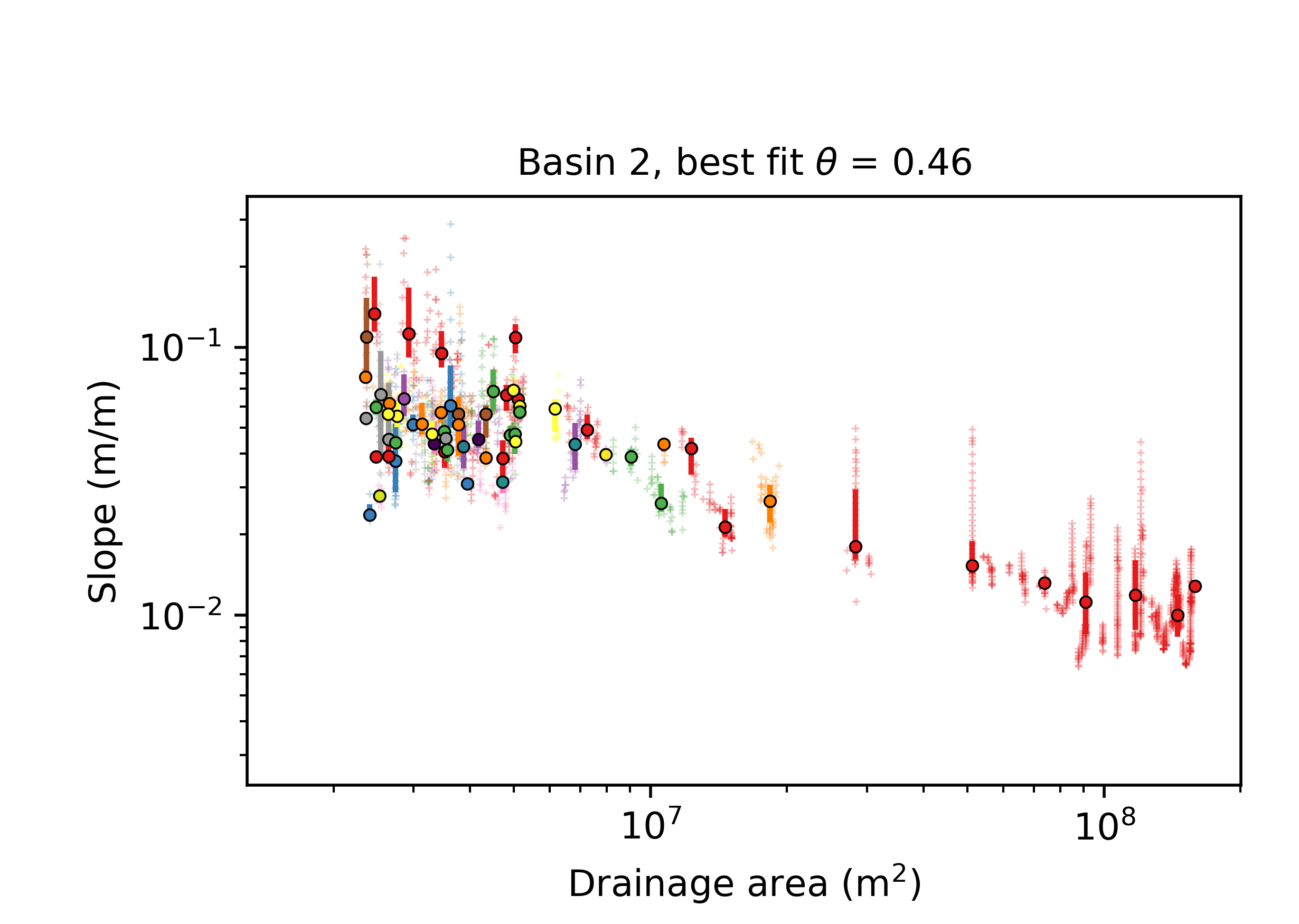  Figure 15. A Slope-area plot in a basin near Xi’an, China. Raw data is in gray symbols. Coloured symbols are log-binned data, with uncertainties, for the main stem (red) and tributaries. Typical problems with Slope-Area data on diplay here: wide scatter in the data, spatial clustering as well as large gaps in drainge area cause by confluences.
4. Chi-elevation profiles for all basins at all tested concavities. The best fit concavities will be labelled in the images. There will be many images in this directory. They look like this:
  
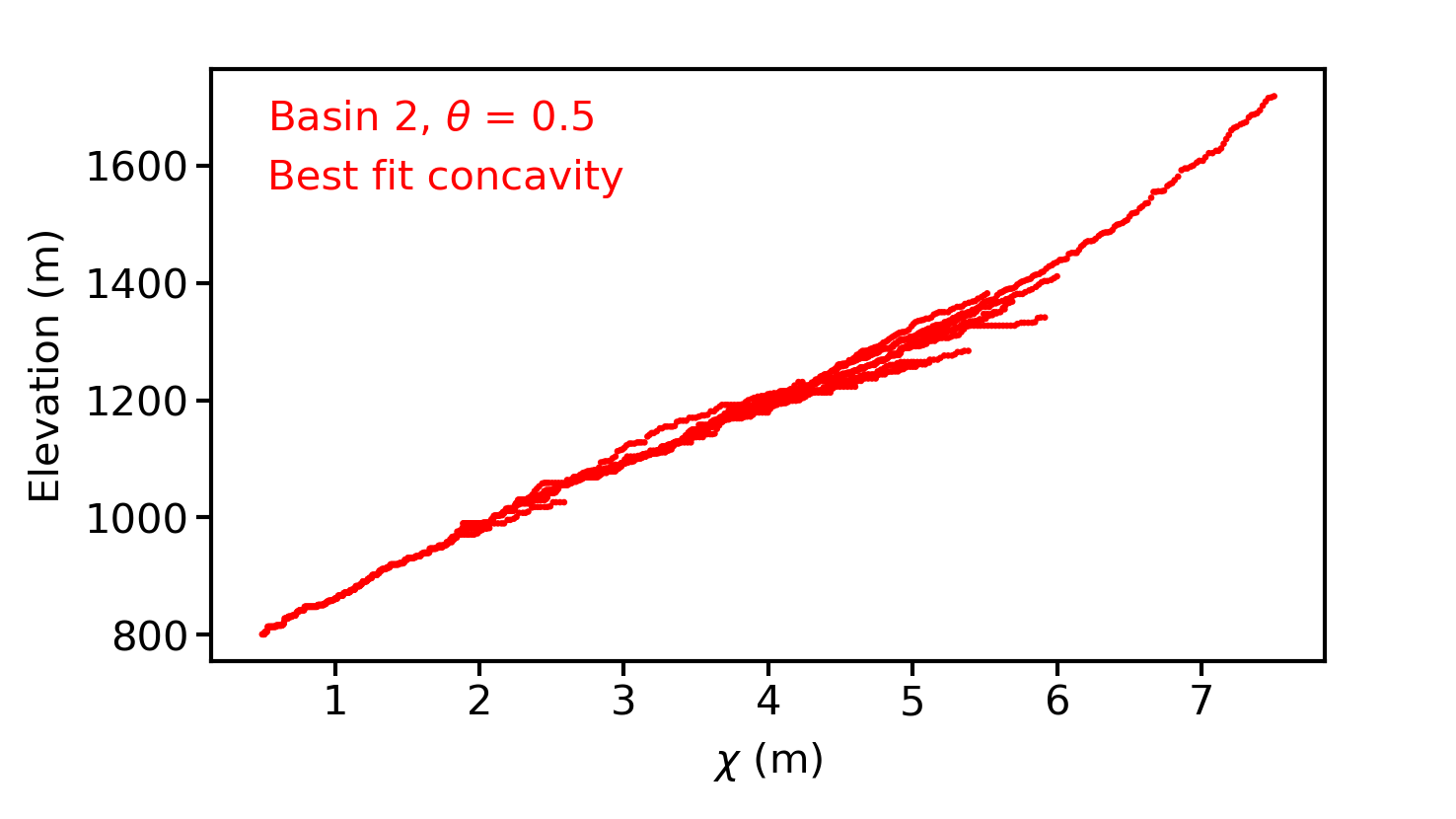  Figure 16. A chi-elevation profile in a basin near Xi’an, China.

Following these steps with your own data (perhaps using Xian_example07.driver as a template) should allow you to do your own concavity analysis on your own landscape. Happy hunting for the best fit concavity!

5.3.4. More options for lsdtt-chi-analysis

There are a number of options in the lsdtt-chi-analysis that are important in generating sensible output for the concavity analysis.

Table 3. Main options for performing a concavity analysis
Keyword	Input type	Default value	Description
estimate_best_fit_movern	bool	false	You need to switch this to `true` to perform all the analysis for channel concavity.
collinearity_MLE_sigma	float	1000	This is a scaling factor for our maximum likelihood estimator (MLE). It does not affect which concavity is the most likely, but does affect the absolute value of MLE. If this value is low, then the MLE values will be zero and you will not get reliable results. If you are getting estimates of concavity that are very low, it might be because sigma is too low. If this is the case you should increase sigma until the best fit values of concavity do not change. In most cases you can use the default but if you have very large networks you may need to increase this parameter. Note that the disorder metrics do not use MLE or the sigma value so changing this has no effect whatsoever on the disorder metrics.
threshold_contributing_pixels	int	1000	This is the minimum number of contributing pixels to form a channel. Lower values will result in denser channel networks.
minimum_basin_size_pixels	int	5000	This is the minimum size of basin in terms of contributing pixels at the outlet.
maximum_basin_size_pixels	int	500000	This is the maximum size of basin in terms of contributing pixels at the outlet.

5.3.5. Other options: all have sensible defaults

There are a number of other options you can choose in the concavity analysis but we have extensively tested the method on dozens of numerical and real test landscapes and the defaults work under most conditions. We encourage users to test the sensitivity of their results to these parameters, but for initial analyses you should not have to change any extra parameters.

5.3.6. What the `estimate_best_fit_movern` routine does

There are two options that wrap all the analyses: * estimate_best_fit_movern * estimate_best_fit_movern_no_bootstrap

These both estimate the concavity, but the latter (wait for it) doesn’t use the bootstrap method. It instead only uses the disorder metric. We found in Mudd et al. (2018) that for most analyses this is probably good enough, but if you are writing a paper that requires a very robust estimate of concavity you might want to use the bootstrap method.

Note that we also found (see figures 6 and 7 in Mudd et al 2018) that extracting the correct concavity using slope-area plots on numerical sandbox experiments (that is, the simplest possible test of a method for extracting concavity) was unreliable and as a result we do not trust slope-area analysis at all.

If you set estimate_best_fit_movern you switch on all the routines for concavity analysis, and plotting of the data. These switches are:

# we need to make sure we select basins the correct way
find_complete_basins_in_window: true
print_basin_raster: true
write_hillshade: true
print_chi_data_maps: true
force_all_basins: true

# run the chi methods of estimating best fit concavity
calculate_MLE_collinearity: true
calculate_MLE_collinearity_with_points_MC: true
print_profiles_fxn_movern_csv: true

movern_disorder_test: true
disorder_use_uncert: true

# run the SA methods of estimating best fit m/n
print_slope_area_data: true
segment_slope_area_data: true

If you set estimate_best_fit_movern_no_bootstrap you do essentially the same thing exept with these changes:

calculate_MLE_collinearity: false
calculate_MLE_collinearity_with_points_MC: false

You can see what these do in the section: Parameter file options.

5.4. Running the concavity analysis

As with all of our tools, we suggest you keep your data and the source code separate. We will assume the standard directory structure described in the section: Installing the code and setting up directories.

We will assume your data is in the folder /LSDTopoTools/Topographic_projects/LSDTT_chi_examples, which you can clone from github.

A very simple driver file is in the example folder, called movern_Xian.driver. This is the driver function:

# Parameters for performing chi analysis
# Comments are preceeded by the hash symbol
# Documentation can be found here:
# https://lsdtopotools.github.io/LSDTopoTools_ChiMudd2014/

# These are parameters for the file i/o
# IMPORTANT: You MUST make the write directory: the code will not work if it doesn't exist.
read path: /LSDTopoTools/Topographic_projects/LSDTT_chi_examples
write path: /LSDTopoTools/Topographic_projects/LSDTT_chi_examples
read fname: Xian
write fname: movern_Xian
channel heads fname: NULL

# We remove parts of the landscape below 400 metres elevation to remove some alluvial fans.
minimum_elevation: 400

# Parameters for selecting channels and basins
threshold_contributing_pixels: 5000
minimum_basin_size_pixels: 150000
maximum_basin_size_pixels: 400000

# Everything you need for a concavity analysis
estimate_best_fit_movern: true

All you need to do is run this file using the chi_mapping_tool. If you followed instructions for installing the software, this tool will be in the directory /LSDTopoTools/Git_projects/LSDTopoTools_. Navigate to that folder:
```
$ cd /LSDTopoTools/Git_projects/LSDTopoTool_ChiMudd2014/driver_functions_MuddChi2014/
```

Now run the correct driver file:

$ ./chi_mapping_tool.exe /LSDTopoTools/Topographic_projects/LSDTT_chi_examples movern_Xian.driver

This might take 5-10 minutes on a reasonable desktop computer.

Congratulations! You have set your first concavity analysis running. It might take a little while to work its way though all the analyses so sit back, relax, and catch up on some important news. When it finishes you will be ready to visualise your data.

5.5. Visualising the results of our concavity analyses

You need to run the analysis before any of this will work!

We have built a single python script that does all the visualisation for you. It works with one call to the script: *easy peasy!!*

Unfortunately there are a few hiccups in getting the python installed, which we describe in a separate section on visualisation.

5.5.1. Generating all the plots

This is a repeat of the example in the previous section, but slightly more general.

Start up the visualisation docker container (native linxu differs, go back to the earlier installation instructions):
```
$ docker run -it -v C:\LSDTopoTools:/LSDTopoTools lsdtopotools/lsdtt_viz_docker
```
Then run Start_LSDTT.sh to download the python tools.
Now go into the LSDMappingTools directory:
```
$ cd /LSDTopoTools/LSDMappingTools/
```

Now run a concavity plotting routine

$ python PlotMOverNAnalysis.py -dir /LSDTopoTools/data/ExampleTopoDatasets/ChiAnalysisData/Xian/ -fname Xian -ALL True

The follow options are required:
1. -dir The directory of your data.
2. -fname The prefx of your data.
The following are optional:
1. -ALL Plots all the concavity plots. Takes a long time! Why don’t you relax and watch a video while you wait?
2. -PC Plots the chi profile plots.
3. -disorder Plots summary plots for the disorder metric. You can run the bootstrap methods but these take a bery long time so you can just stick to disorder plotting in most cases.

5.5.2. What sort of plots do I get?

In your data directory you will now find not one, not two, but four, yes four new directories:

raster_plots
SA_plots
chi_plots
summary_plots

These contain a cornucopia of images for you to explore. Any you got all this for free!! If you use this software you might consider buying Fiona Clubb a coffee or beer when you see her at a conferences given the amount of time she has just saved you by writing these routines.

Figures in the Raster_plots directory

The raster_plots directory contains images of the extracted basins:

Basins around Mount Hua for concavity analysis

Figure 17. The extracted basins for the concavity analysis

It also contains images of the most likely concavity following three methods: slope-area analysis, collinearity analysis of chi profiles using all channel points, collinearity using chi points at random intervals iterated upon using bootstrapping, and collinearity using a disorder metric. Our extensive testing against numerical models under ideal conditions suggest the least trustworthy of these extracted concavity values is the slope-area data, whereas the most trustworthy are the data derived from disorder and bootstrapping approaches. It is not possible to know which of these methods is "true" but if all methods agree you can have high confidence in the concavity and if they disagree our guidance is to use the disorder and bootstrapping methods.

Figure 18. The most likely concavity values using collinearity test of chi profiles with bootstrapping

Figures in the SA_plots directory

This folder contains two versions of slope-area plots. The first contains the slope area data of all the tributaries, for example:

Figure 19. S-A data of all channels in the basin

The second set of S-A data contains only the trunk channel and also has segments extracted from the Mudd et al. (2014) segmentation algorithm.

Figure 20. S-A data of the trunk stream with statistically extracted segments.

Figures in the chi_plots directory

This directory has a large number of images: each chi-elevation plot for each basin for each concavity value tested. If you are seeing interesting patterns in the raster data you should absolutely explore these plots to see what the chi profiles are doing as you vary concavity.

Figure 21. chi plots

Figures in the summary_plots directory

We also print summary plots that let you explore the variation of computed concavity values across a landscape. There are three plots in this directory and two .csv files that contain the underlying data. The three plots are

A plot showing the best fit concavity as a function of basin key that includes the various chi methods and the slope-area method using a regression through all the data.

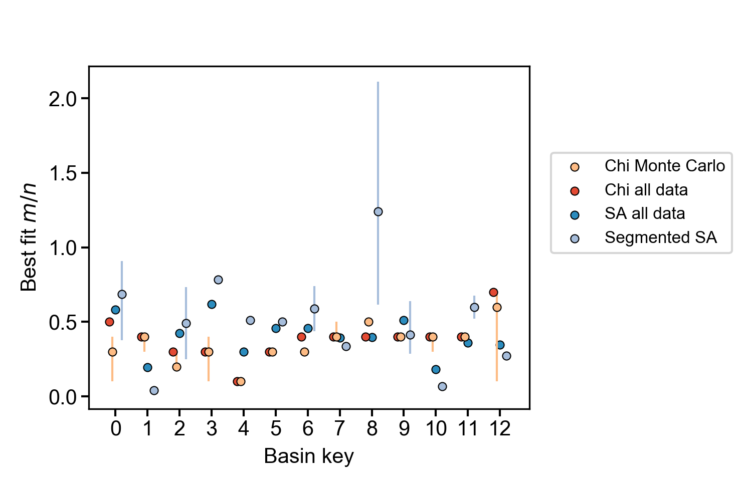Figure 22. Summary plot of most likely concavity ratio for various methods
A plot showing the best fit concavity for just the bootstrap and disorder methods, which we have found to be the most reliable.

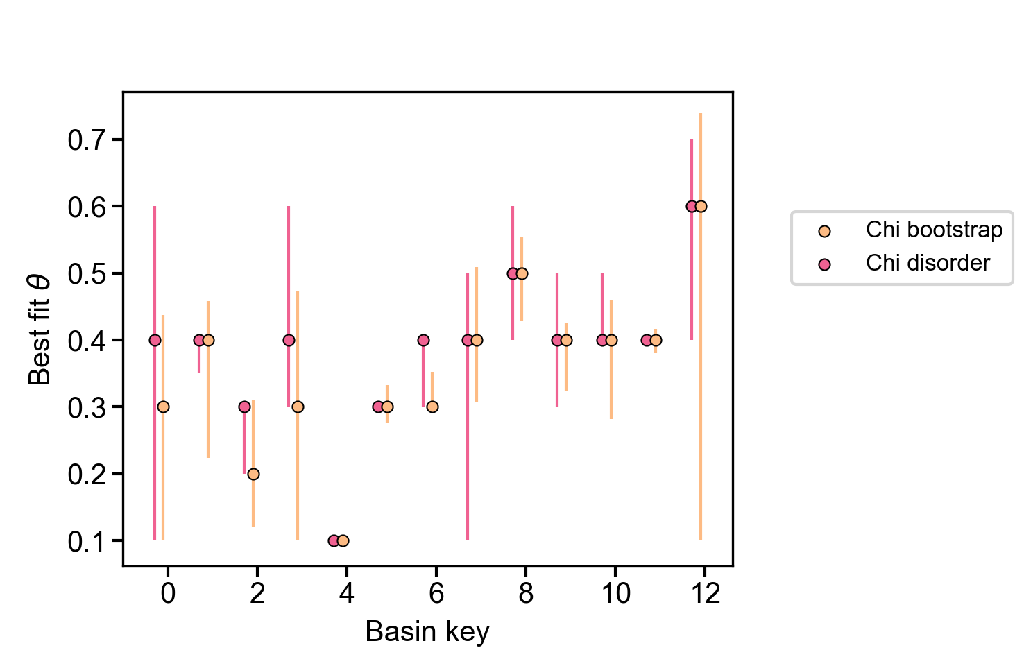Figure 23. Summary plot of most likely concavity ratio for bootstrap and disorder methods
A plot showing the probability of different concavity values of each of the different methods plotted as a Ridgeline plots.

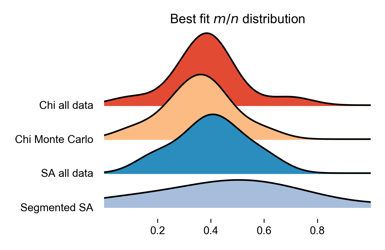Figure 24. Ridgeline plot of the most likely concavity values across all basins in the landscape

5.6. Interpreting results from the concavity analyses and pitfalls

We have tested these routines across a number of landscapes and hope that other workers will find them useful and enhance their own work. Here we explore a number of issues we have come across in interpreting results from these analyses.

5.6.1. Uncertainty and confidence in the results

There are issues in both slope-area analysis and chi-based methods of estimating concavity ($\theta$). S-A data is extremely noisy, whereas the chi method makes some assumptions about how channels erode. In real landscapes, there in no way to test if the extracted concavity value is correct.

We have attempted to understand how well these methods do using numerical models forced to obey the stream power law. This has the obvious drawback that we don’t know if the stream power law is representative of channel erosion processes in any given landscape. But at a minimum we can force a concavity value (in stream power the m/n ratio is equal to the concavity) under idealised, simulated conditions and see how well the methods are able to reproduce the correct concavity.

We have performed a number of simulations where uplift (and thus erosion) rates vary in time, where the n exponent varies between model runs, and where both uplift and erodibility vary in space. The latter two violate assumption of the chi method but in real landscapes many of these assumptions will be violated and we wanted to know if one could still extract reasonable approximations of the concavity.

What we found was that slope area analysis performs the worst when reconstructing concavity values, whereas both our bootstrapped points method and the disorder method perform best. For full reporting of these results please see our upcoming ESURF paper (as of 14-September we are not finished but we hope to submit in October).

For slope-area analysis, we tried to estimate uncertainty initially by getting the uncertainties on the regression coefficients of log S-log A data (we did this with bootstrapping and looking standard uncertainties of regression coefficients found in typical statistical packages). The problem with this is that there are very large numbers of data points and these uncertainty metrics are reduced (i.e. lower uncertainty) as more data is added. So the regression coefficients, according to these metrics, are very certain, but compared to model runs the coefficients are wrong! Our approach has been to estimate concavity for all tributaries, and for segments of the channel network, as well as for all data and for the truck channel, and report all the values. These have very high ranges of values in most landscapes. Overall our recommendation is that if slope area data agrees with chi-based metrics that one can have high confidence in the estimated concavity values but otherwise slope area data should be treated with caution.

For chi-based analyses, we tried several methods. Firstly, we compare the fit between all tributary data and the trunk channel. Since all data is used, there are no measures of uncertainty. This is quite unsatisfying so the second method we used was to randomly select a fixed number of points at fixed locations upstream of the tributary junction, calculate the likelihood based on these points, and iterate using this method several hundred or even thousand times. This allows is to calculate a range of maximum likelihood estimators (MLE) for each concavity value, and we then can calculate the uncertainty bands. We do this by using the minimum MLE value for the most likely concavity value and then seeing where this is equal to the maximum value of MLE for other concavity value.

We also have a chi based disorder metric based on one proposed by Hergarten et al., 2016. We add uncertainty tests to this method: instead of calculating disorder for the entire network we use combinations of tributaries and build a population of lowest channel disorder for all combinations possible of three tributaries and the main stem.

Because the methods are quite different, we are not able to quantify uncertainty in the same way. This means that the uncertainty metrics should be used with extreme caution!

5.6.2. Parameter values that appear to influence results

There are a few parameter values that can influence results.

Basin selection is quite important, especially for chi methods. Our chi methods compare the chi-elevation profiles of tributaries to the trunk channel. This means that if your basin has no or few tributaries you will not get particularly robust results. This is also the case if all of your tributaries are quite short. You can increase the number and length of tributaries by either increasing the basin size (so increasing minimum_basin_size_pixels and minimum_basin_size_pixels) or by reducing the threshold contributing area to initiate a channel (threshold_contributing_pixels).
Avoiding fan surfaces or alluvial surfaces: Our tools are mainly designed for mountain landscapes. Alluvial fans and alluvial channel have different concavities than bedrock channels. In addition, these tend to be low relief surfaces so slope values are very sensitive to topographic errors. By turning remove_seas: true and setting the minimum_elevation to a value that is the approximate elevation of your mountain front.
The collinearity_MLE_sigma should be increased if you are finding that most of your concavity values are coming out as the same, very low value. Sometimes channels have low concavity! But sometimes the MLEs in a basin are all zero and in this case the code defaults to the lowest concavity value given (start_movern). You can tell if channels are actually low concavity by looking at the chi plots.

5.7. Files output by the concavity analysis

The concavity analysis will produce a number of new files in both raster and comma separated value formats. You can also tell the code to print csv files to geojson files if you want to directly load them into your favourite GIS.

We expect most users will go straight to the figures generated by our python script, which should generate dozens of publication quality figures (we have even sized the figures so they are just right for a journal page). However, we list here the file outputs so you can inspect the data outputs with which you can create your own plotting routines, if you so wish. We believe data should be transparent and reproducible, so all our python plots make figures from data that has been printed to file: you will always be able to see the data behind the figures. Please do not abuse our willingness to do this by taking our data and publishing horrible figures created in excel.

5.7.1. Files created by the chi mapping tool

These files will be created by the chi mapping tool and will be located in the directory designated by the read path parameter in the parameter file.

Table 4. Raster files
Filename contains	File type	Description
_hs	raster	The hillshade raster.
_AllBasins	raster	A raster with the basins. The numbering is based on the basin keys.

Table 5. Files used for plotting channels, basins and profiles
Filename contains	File type	Description
_AllBasinsInfo.csv	csv	A csv file that contains some information about the basins and their outlets. Used in our python plotting routines.
_chi_data_map	csv	This contains data for the channel pixels that is used to plot channels, such as location of the pixels (in lat-long WGS1984), elevation, flow distance, drainage area, and information about the basin and source key (the latter being a key to identify individual tributaries). Chi is also reported in this file, it is defaulted to a concavity value = 0.5. To look at profiles with different concavity values use `_movern`
_movern	csv	This prints the chi-elevation profiles. The data includes locations f the channel points, and also chi coordinate for each point for every concavity value analysed.

Table 6. Files containing statistics from chi-based methods
Filename contains	File type	Description
_movernstats_XX_fullstats	csv	Contains the MLE and RMSE values for each tributary in each basin when compared to the trunk stream. Every concavity value has its own file, so if concavity = 0.1, the filename would be called `_movernstats_0.1_fullstats`.
_movernstats_basinstats	csv	This takes the total MLE for each basin, which is the product of the MLE values for each tributary in the basin, and reports these for each concavity value investigated. Essentially collates MLE information from the `_movernstats_XX_fullstats` files.
_MCpoint_XX_pointsMC	csv	This reports on the results from the bootstrap approach. For each concavity value, it samples points for `N` iterations (determined by the `MC_point_iterations` flag) and then calculates summary statistics for each basin. These include minimum, first quartile, median, third quartile and maximum MLE values. Each concavity ratio gets its own file, so if concavity = 1 the file is called `_MCpoint_0.1_pointsMC.csv`.
_MCpoint_points_MC_basinstats	csv	This reports on the results from the bootstrap approach, compiling data from the `_MCpoint_XX_pointsMC.csv`. The file reports on each basin, with the first quartile, median and third quartile reported for every concavity value analysed. Note that now that I have gone through the trouble of writing this documentation it is unlikely these idiotic filenames will change. I take full responsiblity. Mi dispiache. SMM
_movern_residuals_median	csv	This reports the median value of all the residuals of the full chi dataset between tributaries and the trunk stream. The idea here was that the best fit concavity value might correspond to where residuals were evenly distributed above and below the main stem channel. After testing this, however, we found that this always overestimated concavity, so we do not include it in the summary plots. Retained here for completeness. The first and third quartile of residuals are also reported in their own files (`_movern_residuals_Q1` and `_movern_residuals_Q3`).
_fullstats_disorder_uncert	csv	This contains the disorder statistics for every basin. To get this file you need to set `movern_disorder_test: true`. Each basin reports the disorder statistic for every concavity value. The minimum value of disorder is used to select the most likeley concavity.
_fullstats_disorder_uncert	csv	This contains the disorder statistics for every basin. To get this file you need to set `movern_disorder_test: true` and `disorder_use_uncert: true`. The columns are: basin key, the number of combinations (so the number of samples), the minimum, first quartile, median, third quartile and maximum values for best fit concavity (determined with the minimum disorder statistic). It also includes the mean, standard deviation, standard error and MAD for the combination results. Finally, it reports the minimum disorder concavity for all tributaries in the basin (i.e., the minimum disorder if you use all the data).

Table 7. Files associated with slope-area analysis
Filename contains	File type	Description
_SAvertical	csv	This is the slope area data. Slope is calculated over a fixed vertical interval, where the area is calculated in the middle of this vertical interval. The interval is set by `SA_vertical_interval`. The vertical intervals do not cross tributary junctions so there should be no large jumps in drainage area within a vertical interval.
_SAbinned	csv	This is the slope area data averaged into log bins. Summary statistics are provided for each bin (see column headings). The width of the log bins is determined by `log_A_bin_width`.
_SAsegmented	csv	This contains information about the segments in log S- log A space determined by the segmentation algorithm of Mudd et al. 2014. The minimum segment length is set by `slope_area_minimum_segment_length`. Regression statistics (slope, intercept, R²) and Durbin-Watson statistics are reported for each segment.

5.7.2. Files created by the python script PlotMoverNAnalysis.py

These files will be created by PlotMOverNAnalysis.py * and will be in the *summary_plots directory.

Table 8. Summary files
Filename contains	File type	Description
_movern_summary	csv	This contains summary data on the most likely concavity value using a number of different methods. The methods are labelled in the column headers.
_SA_segment_summary	csv	This contains the summary data on the best fit concavity values of slope-area segments in each basin.

5.8. All options used in the concavity analyses

This is a complete list of the options that are used in the concavity analysis. Note that many other options are possible for printing, basin selection and output data formats. You will find all possible options in the section: Parameter file options. What is reported below is just repeated from that section.

5.8.1. Parameters for exploring channel concavity ratio with chi analysis

Table 9. Parameters for trying to constrain concavity using chi analysis
Keyword	Input type	Default value	Description
start_movern	float	0.1	In several of the concavity ($\theta$, or here m/n) testing functions, the program starts at this m/n value and then iterates through a number of increasing m/n values, calculating the goodness of fit to each one.
delta_movern	float	0.1	In several of the concavity ($\theta$, or here m/n) testing functions, the program increments m/n by this value.
n_movern	int	8	In several of the concavity ($\theta$, or here m/n) testing functions, the program increments m/n this number of times.
only_use_mainstem_as_reference	bool	true	If true this compares the goodness of fit between the tunk channel and all tributaries in each basin for each concavity value. If false, it compares all tributaries and the main stem to every other tributary.
print_profiles_fxn_movern_csv	bool	false	If true this loops though every concavity value and prints (to a single csv file) all the chi-elevation profiles. Used to visualise the effect of changing the concavity ratio on the profiles.

Table 10. Different types of concavity tests
Keyword	Input type	Default value	Description
calculate_MLE_collinearity	bool	false	If true loops though every concavity value and calculates the goodness of fit between tributaries and the main stem. It reports back both MLE and RMSE values. Used to determine concavity. This uses ALL nodes in the channel network. The effect is that longer channels have greater influence of the result than small channels.
calculate_MLE_collinearity_with_points	bool	false	If true loops though every concavity value and calculates the goodness of fit between tributaries and the main stem. It reports back both MLE and RMSE values. Used to determine concavity. It uses specific points on tributaries to compare to the mainstem. These are located at fixed chi distances upstream of the lower junction of the tributary. The effect is to ensure that all tributaries are weighted similarly in calculating concavity.
calculate_MLE_collinearity_with_points_MC	bool	false	If true loops though every concavity value and calculates the goodness of fit between tributaries and the main stem. It reports back both MLE and RMSE values. Used to determine concavity. It uses specific points on tributaries to compare to the mainstem. The location of these points is selected at random and this process is repeated a number of times (the default is 1000) to quantify uncertainty in the best fit concavity. We call this the bootstrap method.
collinearity_MLE_sigma	float	1000	A value that scales MLE. It does not affect which concavity is the most likely. However it affects the absolute value of MLE. If it is set too low, MLE values for poorly fit segments will be zero. We have performed sensitivity and found that once all channels have nonzero MLE values the most likely channel does not change. So this should be set high enough to ensure there are nonzero MLE values for all tributaries. Set this too high, however, and all MLE values will be very close to 1 so plotting becomes difficult as the difference between MLE are at many significant digits (e.g., 0.9999997 vs 0.9999996). We have found that a value of 1000 works in most situations.
MC_point_fractions	int	5	For the `calculate_MLE_collinearity_with_points_MC` analysis, this is the number of points on each tributary to test against the main stem channel.
MC_point_iterations	int	1000	For the `calculate_MLE_collinearity_with_points_MC` analysis, this is the number iterations of drawing random points with which to build best fit concavity statistics.
max_MC_point_fraction	float	0.5	The maximum fraction of the length, in chi, of the main stem that points will be measured over the tributary. For example, if the main stem has a chi length of 2 metres, then points on tributaries up to 1 metres from the confluence with the main stem will be tested by the `calculate_MLE_collinearity_with_points_MC` routine.
movern_residuals_test	bool	false	If true loops though every concavity value and calculates the mean residual between the main stem and all the tributary nodes. It is used to search for the concavity value where the residual switches from negative to positive. The rationale is that the correct concavity might be reflected where the mean residual is closest to zero.
movern_disorder_test	bool	false	Test for concavity using the disorder metric similar to that used in Hergarten et al. 2016. Calculates the disorder statistic for each basin while looping through all the concavity values. User should look for lowest disorder value.
disorder_use_uncert	bool	false	This attempts to get an idea of uncertainty on the disorder metric by taking all combinations of 3 tributaries plus the main stem and calculating the disorder metric. Then the best fir concavity for each combination is determined. The best fit concavities from all combinations are then used to calculate minimum, 1st quartile, median, 3rd quartile and maximum values for the least disordered concavity. In addition the mean, standard deviation, standard error, and MAD are calculated. Finally the file produced by this also gives the least disordered concavity if you consider all the tributaries.

Table 11. Parameters for exploring the concavity using Monte Carlo-Markov chain analysis. This is extremely time consuming and doesn’t really produce useful results. Only start if you want to kill your server for nefarious purposes.
Keyword	Input type	Default value	Description
MCMC_movern_analysis	bool	false	If true, runs a Monte Carlo Markov Chain analysis of the best fit m/n. First attempts to tune the sigma value for the profiles to get an MCMC acceptance rate of 25%, then runs a chain to constrain uncertainties. At the moment the tuning doesn’t seem to be working properly!! This is also extremely computationally expensive, for a, say, 10Mb DEM analysis might last several days on a single CPU core. If you want uncertainty values for the m/n ratio you should use the `calculate_MLE_collinearity_with_points_MC` routine.
MCMC_chain_links	int	5000	Number of links in the MCMC chain
MCMC_movern_minimum	float	0.05	Minimum value of the m/n ratio tested by the MCMC routine.
MCMC_movern_maximum	float	1.5	Maximum value of the m/n ratio tested by the MCMC routine.

5.8.2. Parameters for exploring the concavity with slope-area analysis

Table 12. Parameters for exploring the concavity ratio with slope-area analysis
Keyword	Input type	Default value	Description
SA_vertical_interval	float	20	This parameter is used for slope-area analysis. Each channel is traced downslope. A slope (or gradient) is calculated by dividing the fall in the channel elevation over the flow distance; the program aims to calculate the slope at as near to a fixed vertical interval as possible following advice of Wobus et al 2006.
log_A_bin_width	float	0.1	This is for slope-area analysis. The raw slope-area data is always a horrendous mess. To get something that is remotely sensible you must bin the data. We bin the data in bins of the logarithm of the Area in metres². This is the log bin width.
print_slope_area_data	bool	false	This prints the slope-area analysis to a csv file. It includes the raw data and binned data. It is organised by both source and basin so you analyise different channels. See the section on outputs for full details.
segment_slope_area_data	bool	false	If true, uses the segmentation algorithm in Mudd et al., JGR-ES 2014 to segment the log-binned S-A data for the main stem channel.
slope_area_minimum_segment_length	int	3	Sets the minimum segment length of a fitted segment to the S-A data.
bootstrap_SA_data	bool	false	This bootstraps S-A data by removing a fraction of the data (set below) in each iteration and calculating the regression coefficients. It is used to estimate uncertainty, but it doesn’t really work since uncertainty in regression coefficients reduces with more samples and S-A datasets have thousands of samples. Left here as a kind of monument to our futile efforts.
N_SA_bootstrap_iterations	int	1000	Number of boostrapping iterations
SA_bootstrap_retain_node_prbability	float	0.5	Fraction of the data retained in each bootstrapping iteration.

Appendix A: Chi analysis options and outputs

This section is technical and not based on tutorials! It explains the various options and data outputs of the chi mapping tool.

If you want specific examples of usage you may wish to skip to theses sections

Examples of chi analysis
Calculating concavity

A.1. A typical call to lsdtt-chi-mapping

The chi analysis, and a host of other analyses, are run using the lsdtt-chi-mapping program. If you followed the instructions in the section Getting the software you will already have this program compiled.

The program lsdtt-chi-mapping runs with two inputs when you call the program:

In the next section we will walk you though an analysis. However, reading this will help you understand where you are going, so we recommend you read the whole thing!

You run the program from a terminal window
You can supply the program with:
- a directory name
- a parameter file name
- both of these things
- none of these things
If you don’t supply a parameter filename, the program will assume the parameter file is called LSDTT_parameters.driver

If the parameter file doesn’t exist, you will get an error message.

Any of the following calls to one of the programs will work, as long as your files are in the right place:

$ lsdtt-chi-mapping
$ lsdtt-chi-mapping /LSDTopoTools/data/A_project
$ lsdtt-chi-mapping AParameterFile.param
$ lsdtt-chi-mapping /LSDTopoTools/data/A_project AParameterFile.param

A.2. Text editors for modifying files

You will need to modify the parameter file in a text editor. You might also modify python scripts in a text editor. So you need to get a text editor. We use Brackets and Atom (these are platform independent). Sometimes we also use PSPad.

A.3. The parameter file

The parameter file has keywords followed by a value. The format of this file is similar to the files used in the LSDTT_analysis_from_paramfile program, which you can read about in the section [Running your first analysis].

The parameter file has a specific format, but the filename can be anything you want. We tend to use the extensions .param and .driver for these files, but you could use the extension .MyDogSpot if that tickled your fancy.

The parameter file has keywords followed by the : character. After that there is a space and the value.

Chi mapping parameter file format

Lines beginning with # are comments.
Keywords or phrases are followed by a colon (:).
The order of the keywords do not matter.
Keywords are not sensitive, but must match expected keywords.
If a keyword is not found, a default value is assigned.

A.4. Parameter file options

Below are options for the parameter files. Note that all DEMs must be in ENVI bil format (DO NOT use ArcMap’s bil format: these are two different things. See the section Preparing your data if you want more details). The reason we use bil format is because it retains georeferencing which is essential to our file output since many of the files output to csv format with latitude and longitude as coordinates.

A.4.1. Basic file input and output

Table 13. File input and output options. **These do not have defaults and MUST be declared**.
Keyword	Input type	Description
write path	string	The path to which data is written. The code will NOT create a path: you need to make the write path before you start running the program.
read path	string	The path from which data is read.
write fname	string	The prefix of rasters to be written without extension. For example if this is `Test` and you have selected `bil` format then a fill operation will result in a file called `Test_Fill.bil`.
read fname	string	The filename of the raster to be read without extension. For example if the raster is `MyRaster.bil`, read fname will be `MyRaster`.
channel heads fname	string	The filename of a channel heads file. You can import channel heads. If this is set to `NULL` then the channels will be calculated using a pixel threshold.

A.4.2. DEM preprocessing

Table 14. DEM preprocessing. These just help you clean data and perform very basic operations.
Keyword	Input type	Default value	Description
minimum_elevation	float	0	If you have the `remove_seas` keyword set to true, the program will change any elevation node below this value to NoData.
maximum_elevation	float	30000	If you have the `remove_seas` keyword set to true, the program will change any elevation node above this value to NoData.
remove_seas	bool	false	If true, this changes extreme value in the elevation to NoData.
min_slope_for_fill	float	0.001	The minimum slope between pixels for use in the fill function.
raster_is_filled	bool	false	If true, the code assumes the raster is already filled and doesn’t perform the filling routine. This should save some time in computation, but make sure the raster really is filled or else you will get segmentation faults!
only_check_parameters	bool	false	If true, this checks parameter values but doesn’t run any analyses. Mainly used to see if raster files exist.

A.4.3. Selecting channels and basins

Table 15. Options for determining which channels and basins to analyse, including settings for the fill function.
Keyword	Input type	Default value	Description
CHeads_file	string	NULL	This reads a channel heads file. It will supercede the `threshold_contributing_pixels` flag. That is, if you give a valid CHeads filename the code will ignore the threshold pixels and use the sources in the file instead. You can calculate channel heads using our channel extraction tools. The file needs to be a csv file and you pass the filename WITHOUT EXTENSION. The format of the filename is one with 5 columns: `node_index,row,col,x,y`. The `x,y` coordinates are in local UTM coordinates.
BaselevelJunctions_file	string	NULL	This reads a baselevel junctions file. It overrides other instructions for selecting basins. To use this you must have a file with differen junction indices as the outlets of your basins. These can be space separated.
get_basins_from_outlets	bool	false	If this is true the code will look for a file containing the latiitude and longitude coordinates of outlets.
basin_outlet_csv	bool	string	The file containing the outlets. This file must be csv format and have the column headers `latitude` and `longitude`. The coordinates must be in WGS84 (EPSG:4326).
threshold_contributing_pixels	int	1000	The number of pixels required to generate a channel (i.e., the source threshold).
minimum_basin_size_pixels	int	5000	The minimum number of pixels in a basin for it to be retained. This operation works on the baselevel basins: subbasins within a large basin are retained.
maximum_basin_size_pixels	int	500000	The maximum number of pixels in a basin for it to be retained. This is only used by `find_complete_basins_in_window` but that algorithm for selecting basins is the default.
extend_channel_to_node_before_receiver_junction	bool	true	If true, the channel network will extend beyond selected baselevel junctions downstream until it reaches the pixel before the receiver junction. If false, the channel simply extends upstream from the selected basin. The reason for this switch is because if one if extracting basins by drainage order, then the, say, a 2nd order drainage basin starts at the node immediately upstream of the most upstream 3rd order junction.
find_complete_basins_in_window	bool (true or 1 will work)	true	THIS IS THE DEFAULT METHOD! If you don’t want this method you need to set it to false. If this is true, it i) Gets all the basins in a DEM and takes those between the `minimum_basin_size_pixels` and `maximum_basin_size_pixels`. It then removes basins that are influenced by the edge of the DEM, and then removes nested basins. The reason for removing basins draining the edge is that all chi and S-A analysis requires that the basin is complete. If not, your area, and therefore chi coordinate, will be incorrect.
find_largest_complete_basins	bool (true or 1 will work)	false	A boolean that, if set to true, will got through each baselevel node on the edge of the DEM and work upstream to keep the largest basin that is not influenced on its edge by nodata. This only operates if `find_complete_basins_in_window` is set to false!
test_drainage_boundaries	bool (true or 1 will work)	true	A boolean that, if set to true, will eliminate basins with pixels drainage from the edge. This is to get rid of basins that may be truncated by the edge of the DEM (and thus will have incorrect chi values). This only operates if BOTH `find_complete_basins_in_window` and `find_largest_complete_basins` are set to false!, OR if you are using a baselevel junctions file.
only_take_largest_basin	bool (true or 1 will work)	false	If this is true, a chi map is created based only upon the largest basin in the raster.
remove_basins_by_outlet_elevation	bool (true or 1 will work)	false	If this is true, basins will be selected based on their outlet elevation. They values retained will fall into a window between and upper and lower threshold (given in the parameters `lower_outlet_elevation_threshold` and `upper_outlet_elevation_threshold`)
lower_outlet_elevation_threshold	float	0	The upper elevation threshold for selecting basin outlets. The is mainly for chi plot when we are comparing chi coordinates across drainage divides as suggested by Willett et al 2014. This technique does not work at al if the chi coordinate starts at different base levels so one appraoch is to select outles at similar elevations and hope that these represent the same base level.
upper_outlet_elevation_threshold	float	25	The upper elevation threshold for selecting basin outlets. The is mainly for chi plot when we are comparing chi coordinates across drainage divides as suggested by Willett et al 2014. This technique does not work at al if the chi coordinate starts at different base levels so one appraoch is to select outles at similar elevations and hope that these represent the same base level.
print_basin_raster	bool	false	If true, prints a raster with the basins. IMPORTANT! This should be set to true if you want to use any of our python plotting functions that use basin information. Note that if this is true it will also print csv files with basin numbers and source numbers to assist plotting.

A.4.4. Basic data output (before calculating chi)

Table 16. Basic printing operations. For simple rasters and network data that doesn’t require chi analysis.
Keyword	Input type	Default value	Description
convert_csv_to_geojson	bool	false	If true, this converts any csv file (except for slope-area data) to geojson format. This format takes up much more space than csv (file sizes can be 10x larger) but is georeferenced and can be loaded directly into a GIS. Also useful for webmapping. It assumes your raster is in UTM coordinates, and prints points with latitude and longitude in WGS84.
print_raster_without_seas	bool	false	If true, prints a raster that has removed the seas (and very high peaks). This is useful if your NoDataValue is not registering and you use the `minimum_elevation`, `maximum_eleation`, and `remove_seas` flags to correct this. WARNING! This overwrites your original raster.
print_stream_order_raster	bool	false	If true, prints the stream order raster (but printing this to csv is more efficient, use `print_channels_to_csv`).
print_channels_to_csv	bool	false	Prints the channel network to a csv file. Includes stream order and other useful information. Much more memory efficient than printing the whole raster. It prints all channel nodes across the DEM rather than printing nodes upstream of selected basins. If you want to see the channels selected for chi analysis use `print_chi_data_maps`.
print_junction_index_raster	bool	false	If true, prints the junction index raster (but printing this to csv is more efficient, use `print_junctions_to_csv`).
print_junctions_to_csv	bool	false	Prints the junction indices to a csv file. Much more memory efficient than printing the whole raster.
print_fill_raster	bool	false	If true, prints the fill raster.
print_DrainageArea_raster	bool	false	If true, prints the drainage area raster (units are m²).
write_hillshade	bool	false	If true, prints the hillshade raster. The format of this is stupidly different from other printing calls for a stupid inheritance reason. Try to ignore. Most GIS routines have a hillshading options but for some reason they look crappier than our in-house hillshading. I’m not sure why but if you want a hillshade I recommend using this function.

A.4.5. Basic parameters for the chi coordinate

Table 17. Parameters for calculating the chi coordinate.
Keyword	Input type	Default value	Description
A_0	float	1	The A₀ parameter (which nondimensionalises area) for chi analysis. This is in m². Note that when A₀ = 1 then the slope in chi space is the same as the channel steepness index (often denoted by k_s).
m_over_n	float	0.5	The m/n parameter (or concavity index, $\theta$) for calculating chi. Note that if you do any concavity analysis (either `calculate_MLE_collinearity` or `print_profiles_fxn_movern_csv`) this $\theta$ value will be replaced.
threshold_pixels_for_chi	int	0	For most calculations in the chi_mapping_tool chi is calculated everywhere, but for some printing operations, such as printing of basic chi maps (`print_simple_chi_map_with_basins_to_csv`, `print_chi_coordinate_raster`, `print_simple_chi_map_to_csv`) you don’t want chi everywhere (this is especially true when writing a simple csv file) so we have this parameter that sets chi to NoData below these threshold contributing pixels. If this is greater than `threshold_contributing_pixels` it will default to `threshold_contributing_pixels`.
basic_Mchi_regression_nodes	int	11	This works with the basic chi map: segments are not calculated. Instead, a moving window, with a length set by this parameter, is moved over the channel nodes to calculate the chi slope. This method is very similar to methods used to calculate normalised channel steepness (k_sn).

A.4.6. Burning rasters to csv

In some circumstances you might want to "burn" secondary data onto your data of the channel network. One example would be if you had a geologic map and wanted to add the rock type as a column to point data about your channels. These routines will take a raster and will add the data values from that raster to each point in the chi data.

At the moment the burning function only works for the print_chi_data_maps routine.

Table 18. Parameters for burning a raster to csv files.
Keyword	Input type	Default value	Description
burn_raster_to_csv	bool	false	If true, takes raster data and appends it to csv data of channel points.
burn_raster_prefix	string	NULL	The prefix of the raster (without the `bil` extension) that contains the data to be burned. Does not include the directory path. The raster MUST be in the same directory as your input DEM.
burn_data_csv_column_header	string	burned_data	The column header for your burned data. If you want our python plotting tools to be happy, do not give this a name with spaces.
secondary_burn_raster_to_csv	bool	false	This is for a second burn raster. If true, takes raster data and appends it to csv data of channel points.
secondary_burn_raster_prefix	string	NULL	This is for a second burn raster. The prefix of the raster (without the `bil` extension) that contains the data to be burned. Does not include the directory path. The raster MUST be in the same directory as your input DEM.
secondary_burn_data_csv_column_header	string	burned_data	This is for a second burn raster. The column header for your burned data. If you want our python plotting tools to be happy, do not give this a name with spaces.

A.4.7. Integrating lithologic information

In some circumstances you might want to integrate lithologic, structural or tectonic information. For example, you might want to append lithologic data to your channel data in order to explore how channel properties vary by lithology. We call the process of appending data from a raster to channel data (that is in csv of json format) "burning": we take raster data and "burn" it onto csv or json data. Our burning routines work for any raster but we have, in addition, a number of routines that are optimised specifically for geologic data. Outputs are formatted to be ready to use by the LSDMappingTools lithologic-related plotting routines. You can find an automated way to prepare your data from a shapefile in the annexes: [A: Getting your lithologic data ready].

These option are undergoing active development. New options will be regularly added as well as a simplification of the process to prepared the dataset.

Table 19. Parameters for burning a raster to csv files.
Keyword	Input type	Default value	Description
print_litho_info	bool	false	If true, takes a lithologic raster data and appends it to csv data of channel points. It also generates some simple statistic in a csv file called fname_SBASLITH.csv. The routine will also produce a clipped lithology raster with extension `_LITHRAST.bil`.
litho_raster	string	NULL	The prefix of the raster (without the `bil` extension) that contains the geological dataset. Does not include the directory path. The raster MUST be in the same directory as your input DEM. An earlier step is required to generate this file described on another part. The lithology raster DOES NOT need to be the same size as your topographic data. The routine will clip the raster to your topographic raster; this resulting clipped raster will have a filename that contains `_LITHRAST.bil`.

If your lithologic raster is significantly larger than your topographic raster it can result in long loading times, so after the first call to the print_litho_info routine you can replace the litho_raster with fname_LITHRAST (fname will be the name of your DEM) to save computational time.

A.4.8. Parameters for exploring the concavity with chi analysis

Table 20. Parameters for trying to constrain the concavity using chi analysis
Keyword	Input type	Default value	Description
start_movern	float	0.1	In several of the concavity ($\theta$, or here m/n) testing functions, the program starts at this m/n value and then iterates through a number of increasing m/n values, calculating the goodness of fit to each one.
delta_movern	float	0.1	In several of the concavity ($\theta$, or here m/n) testing functions, the program increments m/n by this value.
n_movern	int	8	In several of the concavity ($\theta$, or here m/n) testing functions, the program increments m/n this number of times.
only_use_mainstem_as_reference	bool	true	If true this compares the goodness of fit between the mainstem and all tributaries in each basin for each $\theta$ value. If false, it compares all tributaries and the main stem to every other tributary.
calculate_MLE_collinearity	bool	false	If true loops though every concavity ($\theta$) value and calculates the goodness of fit between tributaries and the main stem. It reports back both MLE and RMSE values. Used to determine $\theta$. This uses ALL nodes in the channel network. The effect is that longer channels have greater influence of the result than small channels.
calculate_MLE_collinearity_with_points	bool	false	If true loops though every concavity ($\theta$) value and calculates the goodness of fit between tributaries and the main stem. It reports back both MLE and RMSE values. Used to determine $\theta$. It uses specific points on tributaries to compare to the mainstem. These are located at fixed chi distances upstream of the lower junction of the tributary. The effect is to ensure that all tributaries are weighted similarly in calculating $\theta$.
calculate_MLE_collinearity_with_points_MC	bool	false	If true loops though every concavity value and calculates the goodness of fit between tributaries and the main stem. It reports back both MLE and RMSE values. Used to determine $\theta$. It uses specific points on tributaries to compare to the mainstem. The location of these points is selected at random and this process is repeated a number of times (the default is 1000) to quantify uncertainty in the best fit $\theta$.
collinearity_MLE_sigma	float	1000	A value that scales MLE. It does not affect which concavity value is the most likely. However it affects the absolute value of MLE. If it is set too low, MLE values for poorly fit segments will be zero. We have performed sensitivity and found that once all channels have nonzero MLE values the most likely channel does not change. So this should be set high enough to ensure there are nonzero MLE values for all tributaries. Set this too high, however, and all MLE values will be very close to 1 so plotting becomes difficult as the difference between MLE are at many significant digits (e.g., 0.9999997 vs 0.9999996). We have found that a value of 1000 works in most situations.
MC_point_fractions	int	5	For the `calculate_MLE_collinearity_with_points_MC` analysis, this is the number of points on each tributary to test against the main stem channel.
MC_point_iterations	int	1000	For the `calculate_MLE_collinearity_with_points_MC` analysis, this is the number iterations of drawing random points with which to build best fit $\theta$ statistics.
max_MC_point_fraction	float	0.5	The maximum fraction of the length, in chi, of the main stem that points will be measured over the tributary. For example, if the main stem has a chi length of 2 metres, then points on tributaries up to 1 metres from the confluence with the main stem will be tested by the `calculate_MLE_collinearity_with_points_MC` routine.
movern_residuals_test	bool	false	If true loops though every concavity ($\theta$) value and calculates the mean residual between the main stem and all the tributary nodes. It is used to search for the $\theta$ value where the residual switches from negative to positive. The rationale is that the correct m/n might be reflected where the mean residual is closest to zero.
print_profiles_fxn_movern_csv	bool	false	If true this loops though every $\theta$ value and prints (to a single csv file) all the chi-elevation profiles. Used to visualise the effect of changing the concavity on the profiles.
movern_disorder_test	bool	false	Test for concavity using the disorder metric similar to that used in Hergarten et al. 2016. Caluculates the disorder statistic for each basin while looping through all the concavity values. User should look for lowest disorder value.
disorder_use_uncert	bool	false	This attempts to get an idea of uncertainty on the disorder metric by taking all combinations of 3 tributaries plus the main stem and calulating the disorder metric. Then the best fir concavity for each combination is determined. The best fit concavities from all combinations are then used to calculate minimum, 1st quartile, median, 3rd quartile and maximum values for the least disordered concavity. In addition the mean, standard deviation, standard error, and MAD are calculated. Finally the file produced by this also gives the least disordered concavity if you conisder all the tributaries.
MCMC_movern_analysis	bool	false	If true, runs a Monte Carlo Markov Chain analysis of the best fit concavity ($\theta$). First attempts to tune the sigma value for the profiles to get an MCMC acceptance rate of 25%, then runs a chain to constrain uncertainties. At the moment the tuning doesn’t seem to be working properly!! This is also extremely computationally expensive, for a, say, 10Mb DEM analysis might last several days on a single CPU core. If you want uncertainty values for the concavity value you should use the `calculate_MLE_collinearity_with_points_MC` routine.
MCMC_chain_links	int	5000	Number of links in the MCMC chain.
MCMC_movern_minimum	float	0.05	Minimum value of the $\theta$ tested by the MCMC routine.
MCMC_movern_maximum	float	1.5	Maximum value of the $\theta$ tested by the MCMC routine.

A.4.9. Parameters for exploring the concavity with slope-area analysis

Table 21. Parameters for exploring the *m/n* ratio with slope-area analysis
Keyword	Input type	Default value	Description
SA_vertical_interval	float	20	This parameter is used for slope-area analysis. Each channel is traced downslope. A slope (or gradient) is calculated by dividing the fall in the channel elevation over the flow distance; the program aims to calculate the slope at as near to a fixed vertical interval as possible following advice of Wobus et al 2006.
log_A_bin_width	float	0.1	This is for slope-area analysis. The raw slope-area data is always a horrendous mess. To get something that is remotely sensible you must bin the data. We bin the data in bins of the logarithm of the Area in metres^2. This is the log bin width.
print_slope_area_data	bool	false	This prints the slope-area analysis to a csv file. It includes the raw data and binned data. It is organised by both source and basin so you analyse different channels. See the section on outputs for full details.
segment_slope_area_data	bool	false	If true, uses the segmentation algorithm in Mudd et al., JGR-ES 2014 to segment the log-binned S-A data for the main stem channel.
slope_area_minimum_segment_length	int	3	Sets the minimum segment length of a fitted segment to the S-A data.
bootstrap_SA_data	bool	false	This bootstraps S-A data by removing a fraction of the data (set below) in each iteration and calculating the regression coefficients. It is used to estimate uncertainty, but it doesn’t really work since uncertainty in regression coefficients reduces with more samples and S-A datasets have thousands of samples. Left here as a kind of monument to our futile efforts.
N_SA_bootstrap_iterations	int	1000	Number of boostrapping iterations
SA_bootstrap_retain_node_prbability	float	0.5	Fraction of the data retained in each bootstrapping iteration.

A.4.10. Parameters for segmentation of channels

Table 22. Parameters for calculating the segments of similar chi slope ($M_{\chi}$). Details can be found in Mudd et al., JGR-ES 2014.
Keyword	Input type	Default value	Description
n_iterations	int	20	The number of iterations of random sampling of the data to construct segments. The sampling probability of individual nodes is determined by the skip parameter. Note that if you want to get a deterministic sampling of the segments you need to set this to 1 and set `skip` to 0. If you are using Monte Carlo sampling you should set this to at least 20 (but probably not more than 100).
target_nodes	int	80	The number of nodes in a segment finding routine. Channels are broken into subdomains of around this length and then segmenting occurs on these subdomains. This limit is required because of the computational expense of segmentation, which goes as the factorial (!!!) of the number of nodes. Select between 80-120. A higher number here will take much longer to compute.
minimum_segment_length	int	10	The minimum length of a segment in sampled data nodes. The actual length is approximately this parameter times (1+skip). Note that the computational time required goes nonlinearly up the smaller this number. Note that this sets the shortest knickzone you can detect, although the algorithm can detect waterfalls where there is a jump between segments. It should be between 6-20.
maximum_segment_length	int	10000	The maximum length of a segment in sampled data nodes. The actual length is approximately this parameter times (1+skip). A cutoff value for very large DEMs.
skip	int	2	During Monte Carlo sampling of the channel network, nodes are sampled by skipping nodes after a sampled node. The skip value is the mean number of skipped nodes after each sampled node. For example, if skip = 1, on average every other node will be sampled. Skip of 0 means every node is sampled (in which case the n_iterations should be set to 1, because there will be no variation in the fit between iterations). If you want Monte Carlo sampling, set between 1 and 4.
sigma	float	10.0	This represents the variability in elevation data (if the DEM has elevation in metres, then this parameter will be in metres). It should include both uncertainty in the elevation data as well as the geomorphic variability: the size of roughness elements, steps, boulders etc in the channel that may lead to a channel profile diverging from a smooth long profile. That is, it is not simply a function of the uncertainty of the DEM, but also a function of topographic roughness so will be greater than the DEM uncertainty.
n_nodes_to_visit	int	10	The chi map starts with the longest channel in each basin and then works in tributaries in sequence. This parameter determines how many nodes onto a receiver channel you want to go when calculating the chi slope at the bottom of a tributary.

A.4.11. Printing of simple chi maps

For most of our visualisation routines, the key printing option to set to true is print_chi_data_maps.

Table 23. Options for printing simple chi maps
Keyword	Input type	Default value	Description
print_chi_coordinate_raster	bool	false	If true, prints a raster with the chi coordinate (in m). Note that if you want to control the size of the data symbols in a visualisation, you should select the `print_simple_chi_map_to_csv` option.
print_simple_chi_map_to_csv	bool	false	If true, prints a csv file with latitude, longitude and the chi coordinate. Can be converted to a GeoJSON with the flag `convert_csv_to_geojson`. This options gives more flexibility in visualisation than the raster, since in the raster data points will only render as one pixel.
print_chi_data_maps	bool	false	This needs to be true for python visualisation. If true, prints a raster with latitude, longitude and the chi coordinate, elevation, flow distance, drainage area, source key and baselevel keys to a csv file with the extension `_chi_data_map.csv`. Many of our visualisation scripts rely on this file.

A.4.12. Chi maps with segmentation and basin and channel selection

Table 24. Options for chi maps and secondary data files that split channels and basins
Keyword	Input type	Default value	Description
print_simple_chi_map_with_basins_to_csv	bool	false	If true, prints a csv file with latitude, longitude and the chi coordinate, as well as basin and source information. Can be converted to a GeoJSON with the flag `convert_csv_to_geojson`. This options gives more flexibility in visualisation than the raster, since in the raster data points will only render as one pixel.
print_basic_M_chi_map_to_csv	bool	false	If true, prints a csv file with latitude, longitude and a host of chi information including the chi slope, chi intercept, drainage area, chi coordinate and other features of the drainage network. The $M_{\chi}$ values are calculated with a rudimentary smoothing window that has a size determined by the parameter `basic_Mchi_regression_nodes`.
print_segmented_M_chi_map_to_csv	bool	false	If true, prints a csv file with latitude, longitude and a host of chi information including the chi slope, chi intercept, drainage area, chi coordinate and other features of the drainage network. The $M_{\chi}$ values are calculated with the segmentation algorithm of Mudd et al. 2014.
print_segments	bool	false	If true, this gives each segment a unique ID that is written to the `segmented_M_chi_map` (use `print_segmented_M_chi_map_to_csv: true`).
print_segments_raster	bool	false	If true, this gives each segment a unique ID and prints to raster. For this to work `print_segments` must be true. We use this to map other landscape metrics, such as various hillslope metrics, to channel segments.
print_source_keys	bool	false	If true, prints a csv file that prints the location of all the channel nodes with each of their source keys. The source keys are just the index into the source numbers: it lets you know which tributary each node belongs to.
print_sources_to_csv	bool	false	This prints as csv that gives information about each of the sources in the DEM. Unless a channel heads csv is provided, these sources will be determined thought a drainage area threshold set by the `threshold_contributing_pixels` flag (default of 1000 pixels).
print_baselevel_keys	bool	false	If true, prints a csv file that prints the location of all the channel nodes with each of their baselevel keys. The baselevel keys are just the index into the baselevel node (i.e., it tells you to which basin each node is connected).

A.4.13. Parameters for dealing with discharge rather than drainage area

These allow the user to drive chi with discharge rather than drainage area. It is somewhat rudimentary at the moment in that it assumes the rainfall rate in length per time is translated into some constant discharge. This is not a hydrological model! It simply accumulates precipitation through a channel network with no regard to hydrological processes, infiltration and evaporation, or the timing of storms.

Table 25. Parameters for dealing with precipitation and discharge.
Keyword	Input type	Default value	Description
precipitation_fname	string	NULL	This is the name (without path or extension) of the precipitation file. There is not much error checking with this file! You MUST pass a file that is the same size as the topography raster!
use_precipitation_raster_for_chi	bool	false	When true, the program will use precipitation to generate a discharge raster and this will be used to calculate chi, rather than drainage area.
print_discharge_raster	bool	false	When true, prints the discharge raster (a convolution of contributing area and precipitation).

A.4.14. Parameters for knickpoint analyses

These parameters drive the knickpoint extraction algorithms.

Table 26. Parameters for dealing with precipitation and discharge.
Keyword	Input type	Default value	Description
ksn_knickpoint_analysis	bool	false	If true, the knickpoint analysis is run. This involves segmenting the chi-elevation data and is therefore quite time consuming.
force_skip_knickpoint_analysis	int	2	Sets the skip for the knickpoint analysis (i.e., not the same as the `skip` parameter).
force_n_iteration_knickpoint_analysis	int	20	Forces the nmber of iterations on the knickpoint analysis.
force_A0_knickpoint_analysis	float	1	Enforces the A_0_ value in the knickpoint analysis.
MZS_threshold	float	0.5	A threshold value for detecting outliers.
TVD_lambda	float	-1	A scaling factor for the TVD analysis on the Mchi values. -1 indicates that the lambda will be set by the concavity. You determine the concavity with our concavity tools. If you get loads of tightly clustered knickpoints it means that the sterm:[k_{sn}] data is very noisy so you will need to increase the $\lambda$ value. The default values of this are (concavity then $\lambda$ pairs): 0.2→0.5, 0.5→20, 0.7→300. So for example if you want fewer tightly clustered knickpoint you may use $\lambda$ = 500 if your concavity is 0.5.
TVD_lambda_bchi	float	10000	A scaling factor for the TVD analysis on the knick intercept. Note that the main variations are extracted on $M_{\chi}$
kp_node_combining	int	10	Determine the combining window for $\Delta k_{sn}$ knickpoint. It avoids getting artifact knickpoints, but a high window can shift knickpoint location. A low window can scatter large knickpoints into successive small ones.
stepped_combining_window	int	20	Forces the nmber of iterations on the knickpoint analysis.
window_stepped_kp_detection	int	100	Determine the window for windowed statistics on segmented elevation to detect stepped knickpoints. Low windows are unefficient to catch these steps.
std_dev_coeff_stepped_kp	float	4	Std deviation threshold to catch these variations. 7 - 9 gives a reasonable results. Lower value would produce many artifacts. 4 is the default

A.5. Example parameter files

We have a number of example parameter files in the repository LSDTT_chi_examples. The chapter on examples will walk you through the various things these files do.

A.6. Output data formats

Data is written to rasters, csv files, or geojson file.

The rasters are all in ENVI bil format, which you can read about in the section: Preparing your data.

ENVI bil should not be mistaken for ESRI bil. Make sure you are using ENVI bil format.
The csv files are comma separated value files which can be read by spreadsheets and GIS software.
- If you import csv files into a GIS you need to tell the GIS about the coordinate system.
- Our csv files all have labeled columns so their contents can be easily views.
- Almost all of our csv files contain latitude and longitude columns. These columns are projected into the WGS84 coordinate system for ease of plotting in GIS software. Select this coordinate system when you loa the csv file into your GIS. For reference it has the EPSG code 4326.
It is very annoying to have to click buttons in a GIS to select a coordinate system each time you look at csv data, so we also allow you to convert to geojson format by using the flag convert_csv_to_geojson in the parameter file.
- The advantage of these files is that they have georeferencing, so you can load them directly into a GIS or web mapping software.
- The disadvantage is that they are HUGE compared to csv files (usually more than 10x the file size). If you are working within GIS software or using web mapping (e.g., d3.js or leaflet) you will probably want to generate these files but if you are using our python plotting tools you can probably forgo creating them.

A.7. The different outputs and how to get them

To get the various outputs, you need to tell the chi mapping tool using the parameter file. These tables tell you what flags to use and what data you will get.

A.7.1. Raster output

Table 27. These are basic rasters that don’t require chi analysis.
parameter file switch	Filename contains	Description
write hillshade: true	_hs.bil	This prints a hillshade raster. Seems to give better results than hillshade functions in GIS software. Also much faster. Much of our plotting tools make nice looking maps when you drape hillshade over elevation data so we suggest you turn this on the first time you analyse a landscape.
print_fill_raster: true	_fill.bil	This prints the fill raster. Filling is computationally expensive so you can do this the first time you run a DEM and then use the `raster_is_filled` flag later to speed up computation.
print_DrainageArea_raster: true	_DArea.bil	This prints the drainage area raster. Drainage area is calculated using the Fastscape D8 flow routing algorithm.
print_basin_raster: true	_AllBasins.bil	This prints a basin raster. Each basin gets an integer value that is keyed to the baselevel. These correspond to the `baselevel_key` that appears in csv data files.
print_chi_coordinate_raster: true	_chi_coord.bil or _chi_coordQ.bil	This prints the chi coordinate. It uses the A₀ and m/n values set by the `A_0` and `m_over_n` flags in the parameter file (defaults are 1 m² and 0.5, respectively). The raster will calculated chi using drainage area, which results in the _chi_coord.bil file, unless the switch `use_precipitation_raster_for_chi` is set to true, in which case a discharge will be calculated from a precipitation raster and this discharge will be used to calculate chi, resulting in a _chi_coordQ.bil file.
print_discharge_raster: true	_Q.bil	If `use_precipitation_raster_for_chi` is set to true, the discharge will be calculated and printed to a raster. Note that there is no real hydrology in this calculation: one should think of it as a number representing the relative supply of water along the channel network. "Discharge" is calculated simply by accumulating the volume of precipitation from each pixel, so precipitation is supplied in m/yr and "discharge" is in m³/yr.
print_chi_no_discharge: true	_chi_coord.bil	Used only if you have set `use_precipitation_raster_for_chi` and `print_chi_coordinate_raster` to true, and you want a chi coordinate raster that is based on drainage area in addition to one based on discharge. Used for comparison purposes, so you can see how big of a change spatially heterogeneous precipitation causes to the chi coordinate.
print_litho_info: true Follow intructions on Integrating lithologic information	_LITHRAST.bil	Automated generation of a clipped lithologic raster to simplify plotting routines.

A.7.2. Point data (usually output as csv)

The table below gives a brief description of the output files. After the table we show the format for each of these files.

If the convert_csv_to_geojson flag is set to true then the csv data headers will be recast as geojson point attributes.

Table 28. Point data available in csv or geojson format. Switch to true to turn on.
parameter file switch, and the filename will contain	Description	Data columns
print_channels_to_csv _CN.csv	Prints the channel network to csv.	latitude,longitude,Junction Index,Stream Order,NI NI is the node index (an index into individual pixels in the DEM), and Junction Index is an index into the `LSDJunctionNetwork` object. Latitude and longitude are in WGS84.
print_junctions_to_csv _JN.csv	Prints junction numbers to csv.	junction,node,x,y,latitude,longitude,stream_order junction is the junction index. Latitude and longitude are in WGS84, whereas x and y are in the local UTM coordinates.
print_sources_to_csv _ATsources.csv	Prints the sources to csv.	node,x,y,latitude,longitude node is the node index from `LSDFlowInfo`. Latitude and longitude are in WGS84, whereas x and y are in the local UTM coordinates.
print_simple_chi_map_to_csv _chi_coord.csv	Prints a very basic chi map.	latitude,longitude,chi Latitude and longitude are in WGS84, chi is in metres.
print_simple_chi_map_with_basins_to_csv _chi_coord_basins.csv	Prints a very basic chi map, but includes the basin.	latitude,longitude,chi,basin_junction Latitude and longitude are in WGS84, chi is in metres. The basin_junction refers to the junction number of the baselevel junction for each node. Allows one to plot these profiles by basin.
print_basic_M_chi_map_to_csv _MChiBasic.csv	This is a very rudimentary version of a map of chi slope (if A₀ = 1, then this is the same as the channel steepness index). No segmentation is performed, it simply calculates chi slope from smoothed profiles.	latitude,longitude,chi,elevation,flow distance,drainage area,m_chi,b_chi,source_key,basin_key Latitude and longitude are in WGS84, chi and flow distance are in metres. Drainage area is in m². M_chi is the slope in chi space, equivalent to k_sn if A₀ is set to 1. b_chi is the intercept of the chi segment. The source_key and basin_key are indices into the basins and sources.
print_segmented_M_chi_map_to_csv _MChiSegmented.csv	This uses segmentation to calculate chi slopes (if A₀ = 1, then this is the same as the channel steepness index) following the Mudd et al, 2014 algorithms.	latitude,longitude,chi,elevation,flow distance,drainage area,m_chi,b_chi,source_key,basin_key Latitude and longitude are in WGS84, chi and flow distance are in metres. Drainage area is in m². M_chi is the slope in chi space, equivalent to k_sn if A₀ is set to 1. b_chi is the intercept of the chi segment. The source_key and basin_key are indices into the basins and sources.
print_segments _MChiSegmented.csv	This uses segmentation to calculate chi slopes (if A₀ = 1, then this is the same as the channel steepness index) following the Mudd et al, 2014 algorithms. It includes the segment data including a segment number and the fitted segment elevation	latitude,longitude,chi,elevation,flow distance,drainage area,m_chi,b_chi,source_key,basin_key,segmented_elevation,segment_number Latitude and longitude are in WGS84, chi and flow distance are in metres. Drainage area is in m². M_chi is the slope in chi space, equivalent to k_sn if A₀ is set to 1. b_chi is the intercept of the chi segment. The source_key and basin_key are indices into the basins and sources. The segmented_elevation is the elevation of the segment, and the segment_number is an increasing integer for each segment. The segment number is used to search for knickpoints if `skip` is set to 0 and `n_iterations` is set to 1.
check_chi_maps _checkchi.csv and _checkchiQ.csv	This is used with the discharge-based chi calculation to compare chi values using discharge (`_checkchiQ.csv`) vs drainage area (`_checkchi.csv`).	latitude,longitude,chi,elevation,flow distance,drainage area,source_key,basin_key Latitude and longitude are in WGS84, chi and flow distance are in metres. Drainage area is in m². The source_key and basin_key are indices into the basins and sources.
print_source_keys _SourceKeys.csv	This prints information about source keys for each node in the channel network. Allows visualisation tools to link nodes to their sources, and thus used to plot tributaries.	latitude,longitude,source_node,source_key Latitude and longitude are in WGS84. The source_node is the node id of the source from the `LSDFlowInfo` object and the source_key is a key of the source (used so that sources are numbered 0,1,2,3, etc. instead of some random large integer).
print_baselevel_keys _BaselevelKeys.csv	This prints information about baselevel keys for each node in the channel network. Allows visualisation tools to link nodes to their baselevel, and thus used to plot basins.	latitude,longitude,baselevel_node,baselevel_junction,baselevel_key Latitude and longitude are in WGS84. The baselevel_node is the node id of the source from the `LSDFlowInfo` object. The baselevel_junction is the junction index from the `LSDJunctionIndex` object, and the baselelvel_key is a key of the baselevel (used so that basins are numbered 0,1,2,3, etc. instead of some random large integer).
print_profiles_fxn_movern_csv _movernQ.csv or _movern.csv	Loops through m/n values and records the chi coordinate for all the channels for each m/n. If `use_precipitation_raster_for_chi` is true then this prints a _movernQ.csv, and prints _movern.csv otherwise.	source_key,basin_key,elevation,m_over_n = 0.2, m_over_n = 0.3, etc. The source_key and basin_key are indices into the basins and sources. elevation is the, wait for it, elevation. Following this there are columns of the chi coordinate for each m/n value, which are determined by the parameters `n_movern`, `start_movern`, and `delta_movern`.
calculate_MLE_collinearity _movernstats or _movernstatsQ with _basinstats.csv	Loops through m/n values and records the goodness of fit between tributaries and main stem for all the channels for each m/n. If `use_precipitation_raster_for_chi` is true then this prints *movernstatsQ* files, and prints *movernstats* otherwise. Generates a large number	basin_key,m_over_n = 0.2, m_over_n = 0.3, etc. The basin_key is and index into the basins and sources. elevation is the, wait for it, elevation. Following this there are columns of the maximum likelihood estimator (MLE) for each basin for each m/n value, which are determined by the parameters `n_movern`, `start_movern`, and `delta_movern`. The higher the MLE, the better the fit. Calculated by projecting each tributary data point onto a linear fit between adjacent nodes in chi-elevation space of the main stem channel.
calculate_MLE_collinearity *movernstats* or _movernstatsQ* with _X_fullstats.csv where X is _m/n*	Loops through m/n values and records the goodness of fit between tributaries and main stem for all the channels for each m/n. These are separate files for each m/n value (denoted in the filename). If `use_precipitation_raster_for_chi` is true then this prints *movernstatsQ* files, and prints *movernstats* otherwise. Generates a large number of files.	reference_source_key,test_source_key,MLE,RMSE The reference_source_key is key of the channel that serves as a reference, against which goodness of fit will be measured. The test_source_key is the source key of the tributary which is being compared to the reference channel. The MLE is the maximum likelihood estimator, where better goodness of fit results in higher numbers, and the RMSE is the root mean square error, where smaller numbers indicate a better fit.
print_litho_info: true _SBASLITH.csv	This simple statistics about the geological content of each of the selected basins, percentages and count of each lithologies.	method,basin_key,one column per geology,total The method is raw count or percentages. The basin_key is the indices into the selected basins. One column per geology codes are then generated and the correspondance between the geology code and your shapefile is explain in the annex TO ADD.

Appendix B: Preparing lithologic data

This appendix explains how to use our python routines to prepare lithology shapefiles for use in LSDTopoTools.

B.1. Getting your lithologic data ready

Lithologic datasets need to be formatted prior to ingestion by LSDTopoTools. At the moment, LSDTopoTools is only to ingest this data in raster format, whereas most lithologic data is provided in shapefiles. We have created a number of python scripts for converting shapefile data into rasters that can be used by LSDTopoTools. Our lithologic routines in LSDTopoTools use an integer key for each rock type, so our python routines manage the conversion of rock types, usually presented as stings, into integer rock types. It will also creae csv keys that allow you to convert back to rock types in plotting routines (e.g., "granite" instead of "7"). The code will then format the raster with the right extent to _LITHRAST.bil. Your lithokey file needs to have a name finishing with _lithokey.csv and needs to have the following headers: ID, containing the data string, and rocktype, containing the corresponding value in the raster. For instance:

_beverley_lithokeys.csv_
ID,rocktype
sandstone,4
granite,2
basalt,1

You can geenrate these lithologic keys manually, but formatting errors can easily be made. We propose there a method to generate automatically all these file with the right format from a shapefile containing the geological information. Here we present python scripts for manageing this process. You will need Python to use the generating script, you can refer to the [Using python] section for instruction about installation.

B.1.1. The `Rasterization.py` script

The Python script that automates this process is present in the LSDMappingTools plotting library developped in parallel of LSDTopoTools. You can refer to the section [Getting our plotting tools] to download the needed repository. The script is Rasterization.py and can be executed using the command line (you do not need to edit the code).

The first step is to open a terminal and to navigate with cd until your *LSDMappingTools folder. You can then obtain the documentation of this script by running the command python Rasterization.py -h displaying the following results:

-h, --help            show this help message and exit
  -dir DIRECTORY, --directory DIRECTORY
                        The base directory with the shapefile. If this isn't
                        defined I'll assume it's the same as the current
                        directory.
  -fn FNAME_PREFIX, --fname_prefix FNAME_PREFIX
                        The name of your shapefile without extention (no .shp
                        at the end)
  -fd FIELD_NAME, --field_name FIELD_NAME
                        The name of the field that will give the value to the
                        raster
  -rast RASTERIZATION, --rasterization RASTERIZATION
                        Rasterize your file into a tif raster and produce a
                        lithokey csv file containing the keys for the
                        numerisation of the data.
  -rn RENAME, --rename RENAME
                        rename your raster after rasterization, optional.
  -UTM UTM_CODE, --UTM_CODE UTM_CODE
                        Give the UTM UTM_CODE of your zone to automate the
                        conversion of the raster into an LSDTopoTools
                        compatible raster.
  -S SOUTH, --SOUTH SOUTH
                        Turn to True if your UTM zone is in the southern
                        hemisphere. A quick way to check that is to go on
                        field and to observe how flow the water in a
  -res RESOLUTION, --resolution RESOLUTION
                        Precise this argument if you want to change the raster
                        resolution, default 30

B.1.2. `Rasterization.py` basic usage

The script needs, at minimum, the following options:

The directory where your shapefile is.
The prefix of the shapefile.
The name of the field containing the information you want to digitise. Almost every geological survey has a different naming convention for rock type. You will need to look at the lithologic data in a GIS and determine the name of the field where the rock type is located. This is case sensitive. This step is easy to break since the field name needs to exactly match the field name in the shapefile.

You can launch the following command to produce a basic rasterization.

$ python Rasterization.py -dir /home/PhilCollins/DataStore/GIS/US/ -fn beverly_litho -fd geology

This command creates a raster and a csv file. However, the output raster will be in WGS94 geographic system.

B.1.3. `Rasterization.py` to output into UTM coordinates

You would need to translate it in UTM to make it usable by LSDTopoTools. You can either use GDAL, your favorite GIS or adding the following options to the python script: -UTM, followed byt the UTM zone of your area, with -S True if your area is in the southern hemisphere. Finaly, you can add at any point the -res X option to set a resolution different than 30 meters and -rn X if you want to specifiy a new name for the raster. A complete command would then be:

python Rasterization.py -dir /home/PhilCollins/DataStore/GIS/Africa/ -fn Tanzania_litho -fd LITH -UTM 33 -SOUTH True -rn GeoRast -res 12

Your raster is then ready to be ingested by LSDTopoTools.

Keyword	Input type	Default value	Description
start_movern	float	0.1	In several of the concavity (\(\theta\), or here m/n) testing functions, the program starts at this m/n value and then iterates through a number of increasing m/n values, calculating the goodness of fit to each one.
delta_movern	float	0.1	In several of the concavity (\(\theta\), or here m/n) testing functions, the program increments m/n by this value.
n_movern	int	8	In several of the concavity (\(\theta\), or here m/n) testing functions, the program increments m/n this number of times.
only_use_mainstem_as_reference	bool	true	If true this compares the goodness of fit between the tunk channel and all tributaries in each basin for each concavity value. If false, it compares all tributaries and the main stem to every other tributary.
print_profiles_fxn_movern_csv	bool	false	If true this loops though every concavity value and prints (to a single csv file) all the chi-elevation profiles. Used to visualise the effect of changing the concavity ratio on the profiles.