Hillslope metrics in LSDTopoTools

Return to main LSDTopoTools landing page

1. Introduction to advanced hillslope analysis

Basic hillslope metrics

If you are looking for basic metrics like slope, curvature and aspect, you should follow the link below:

Basic topographic analyis in LSDTopoTools

In this document we will explore the analysis of hillslopes. The analyses here go beyond simple metrics like curvature and slope, and look at more subtle features of the landscape like channel length and dimensionless relief and curvature. We have used these metrics to understand both sediment flux laws as well as the tectonic evolution of landscapes.

Before you start

Before you start you need to install LSDTopoTools. If you haven’t done that, please follow the link below.

Instructions on how to install LSDTopoTools

In addition, you will need to use some basic linux shell commands. If you have never done this before I suggest reading this brief introduction: Basic use of the linux shell.

1.1. Background reading

If you wish to explore some background reading, a good place to look at how topography can be used to test theories about sediment transport is a series of papers by Josh Roering and colleagues:

We used some of the concepts in those papers to show that ridgetop curvature was a useful metric to quantfy erosion rates as well as find signals of landscape transience:

To understand landscape transience, and also explore sediment flux laws, hillslope length must also be known, and we have developed methods for quantifying hillslope lengths and linking them to ridgetop curvature:

2. Coupling hillslope and channel analysis

Hillslope erosion and the evolution of hillslope morphology though time is often driven by incision or deposition in channels. Tectonic signals can migrate upstream in channels in the form of knickpoints and knickzones, and as these pass the baes of a hillslope, the hillslope will begin to adjust from the base upwards. This can create complex spatial patterns in topographic metrics that may be used to decipher transient changes in the erosion of upland landscapes.

We have developed a series of tools for quantifying the spatial correspondence between channel steepness and hillslope properties. Included in LSDTopoTools2 is a program called lsdtt-hillslope-channel-coupling, which packages routines our group uses to detect coupled channel and hillslope evolution.

The code does a number of things.

It does basic analyses that replicates some of the functionality of lsdtt-basic-metrics and lsdtt-chi-mapping programs. In short, it can calculate surface fitting rasters such as slope, curvature and aspect, and it can extract the chi coordinate (a flow length normalised for drainage area).
- If you want more information on lsdtt-basic-metrics, follow the instructions for basic LSDTT usage
- If you want more information on lsdtt-chi-mapping, follow the instructions for LSDTT chi analyis
It extracts ridgelines from a DEM and has various algorithms for filtering thses ridgelines. It also has algoirthms for splitting ridgelines into segments to perform some spatial averaging if that is what you want to do.
It can perform hilltop flow routing, where flow routing is performed from the hilltops to either the channel, a floodplain, or a buffered channel network in order to link hilltop pixles to channel pixels.
It extracts basic channel networks and then can segment the channel network so that ridgetop pixels can be tagged against channel segments.
It then calculates a range of metrics associated with these hilltop traces. These include dimensionless relief (R*), dimensionless curvature (E*), and hillslope length.

These metrics can tell you quite a lot about the state of the landscape and we feel quite strongly that combining the hillslope and channel metrics can yeild a much richer picture of a landscape’s evolution than either channel or hillslope metrics alone. We very much hope that you will be able to apply these analysis tools to your own landscape. Below we provide some papers that can help you understand what the metrics mean.

Table 1. Relevant publications for understanding what relief and curvature metrics mean
Reference	Description
Roering et al., 2007	This was the initial publication that set out the theory of E* vs R* analysis.
Hurst et al., 2012	This paper explored the relasionship between ridgetop curvature and first speculated as to the response of landscapes to transient incison in E* vs R* space.
Hurst et al., 2013	This paper demonstrated that one could detect landscape transience using ass:[E] vs R data.
Grieve et al., 2016	This paper automated extraction of E* R* metrics
Hurst et al., 2019	The first publication that combines E* R* analysis with channel metrics. These instructions will walk you through running the coulpled hillslope-channel analysis and explain the outputs of the code.

2.1. Getting LSDTopoTools2

The lsdtt-hillslope-channel-coupling program sits within LSDTopoTools2. You can follow our installation instructions.

If you have installed LSDTopoTools2 you will already have hillslope channel coupling routines, as well as the other programs necessary for carrying out the hillslope and channel analysis.

2.2. Running the analysis

This analysis is perhaps the most complex thing you can do with LSDTopoTools. It requires a number of different components to be pulled together for the final product, and it works in a few steps because you need the output of one step to set the parameters for the next steps. So please be patient.

Here are the steps you need to follow:

You need to extract the channel network. It is actually important to get a proper channel network rather than just using some threshold drainge area, because the analysis is more robust if you are comparing basins of similar order and you can’t do that if you don’t know where the channels begin.
If you want, you can use that network to decide on the basins you want to explore. But you can also do that algorithmically.
You then need to determine the concavity of the channels because at some point you are going to calculate the steepness of the channels and for this you need a concavity. If you just need a first cut you can use 0.45, but we have tested for concavity in very many places and can assure you that it is highly variable.
Once you do those things you can then run the hillslope code. Be warned: this last step can take A VERY LONG TIME.

2.3. Get the example data

If you followed the installation instructions you will already have the example data.
It is in (int the docker container) /LSDTopoTools/data/ExampleTopoDatasets/ChannelExtractionData/Guadalupe_1m

2.4. Coupled hillslope and channel ananylsis: options and outfiles

2.4.1. Input options

Like all LSDTopoTools programs, you can set parameters in the lsdtt-hillslope-channel-coupling that drive the analysis. Many of these are shared with other programs in the LSDTopoTools analysis suite.

Basic file input and output

Table 2. File input and output options. **These do not have defaults and MUST be declared**.
Keyword	Input type	Description
THIS IS NOT A KEYWORD	Null	If you don’t enter the write path, read path or write fname, the program will assume that the read and write paths are the current directory, and the write fname is the same as the read fname.
write path	string	The path to which data is written. The code will NOT create a path: you need to make the write path before you start running the program.
read path	string	The path from which data is read.
write fname	string	The prefix of rasters to be written without extension. For example if this is `Test` and you have selected `bil` format then a fill operation will result in a file called `Test_Fill.bil`.
read fname	string	The filename of the raster to be read without extension. For example if the raster is `MyRaster.bil`, read fname will be `MyRaster`.

DEM preprocessing

Table 3. DEM preprocessing. These just help you clean data and perform very basic operations.
Keyword	Input type	Default value	Description
minimum_elevation	float	0	If you have the `remove_seas` keyword set to true, the program will change any elevation node below this value to NoData.
maximum_elevation	float	30000	If you have the `remove_seas` keyword set to true, the program will change any elevation node above this value to NoData.
remove_seas	bool	false	If true, this changes extreme value in the elevation to NoData.
min_slope_for_fill	float	0.001	The minimum slope between pixels for use in the fill function.
raster_is_filled	bool	false	If true, the code assumes the raster is already filled and doesn’t perform the filling routine. This should save some time in computation, but make sure the raster really is filled or else you will get segmentation faults!
only_check_parameters	bool	false	If true, this checks parameter values but doesn’t run any analyses. Mainly used to see if raster files exist.

Hilltop parameters

Table 4. These are used to select hilltops
Keyword	Input type	default	Description
StreamNetworkPadding	int	0	The number of pixels you want to pad the channel network. If a hillslope trace comes within this many pixels of the channel, the trace stops.
min_stream_order_to_extract_basins	int	0	Minimum stream order for extracting basins (or the hilltops of those basins)
max_stream_order_to_extract_basins	int	100	Maximum stream order for extracting basins (or the hilltops of those basins)
RemovePositiveHilltops	bool	true	Remove hilltops with positive curvature (i.e., that are concave)
RemoveSteepHilltops	bool	true	Remove hilltops that are steep. This is because steep (plunging) ridgetop will move into the nonlinear sediment transport regime and there will no longer be a linear relasionship between curvature and erosion rate at steady state. Basically if hilltops are too steep the assumptions of the analysis break down.
Threshold_Hilltop_Gradient	float	0.4	If `RemoveSteepHilltops` is `true`, then any hillslopes steeper than this will be removed.
MaskHilltopstoBasins	bool	true	Need to ask Martin what this does.

Hilltop analysis and printing options

Table 5. These are the different analyses and write options for the hilltops
Keyword	Input type	default	Description
run_HFR_analysis	bool	false	If true, run the entire hilltop flow routing analysis.
write_hilltops	bool	false	If true, write a raster of all the hilltops.
write_hilltop_curvature	bool	false	If true, write a raster of hilltop curvature.
write_hillslope_gradient	bool	false	If true, write a raster of all hillslope gradient
write_hillslope_length	bool	false	If true, write a raster of all hillslope length
write_hillslope_relief	bool	false	If true, write a raster of all hillslope relief
print_hillslope_traces	bool	false	If true, this writes the hillslope traces. Be warned: this is VERY computationally intensive.
hillslope_trace_thinning	int	1	A thinning factor. If it is 1, it writes everyu trace. If 2, every 2nd trace, if 3, ever thrid trace. And so on.
hillslope_traces_file	string	""	The name of the hillslope traces file
hillslope_traces_basin_filter	bool	false	I’m not sure what this does. Ask Martin or Stuart.

Filenames for channel heads, floodplains, and other pre-computed data

Table 6. Options for determining which channels and basins to analyse, including settings for the fill function.
Keyword	Input type	Default value	Description
ChannelSegments_file	string	NULL	A file that has computed the channel segment numbers so that these segments can be linked to ridgetops. It is calculated UPDATE
Floodplain_file	string	NULL	A file that has 1 for floodplain and 0 elsewhere. Used to mask the floodplains so that hillslopes stop there. The format is UPDATE
CHeads_file	string	NULL	This reads a channel heads file. It will supercede the `threshold_contributing_pixels` flag. That is, if you give a valid CHeads filename the code will ignore the threshold pixels and use the sources in the file instead. You can calculate channel heads using our channel extraction tools. The file needs to be a csv file and you pass the filename WITHOUT EXTENSION. The format of the filename is one with 5 columns: `node_index,row,col,x,y`. The `x,y` coordinates are in local UTM coordinates.
BaselevelJunctions_file	string	NULL	File containing a list of baselevel junctions to determine basins to analyse. The basin numbers should be on individual lines of the text file. You can see the junction numbers by printing the junction numbers to a csv with the command `print_junctions_to_csv`.

Selecting channels and basins

There are a number of options for selecting channels and vasins. The basin selection is linked to extracting channel profile analysis and is not used for hillslop analysis.

Table 7. Options for determining which channels and basins to analyse, including settings for the fill function.
Keyword	Input type	Default value	Description
threshold_contributing_pixels	int	1000	The number of pixels required to generate a channel (i.e., the source threshold).
minimum_basin_size_pixels	int	5000	The minimum number of pixels in a basin for it to be retained. This operation works on the baselevel basins: subbasins within a large basin are retained.
maximum_basin_size_pixels	int	500000	The maximum number of pixels in a basin for it to be retained. This is only used by `find_complete_basins_in_window` but that algorithm for selecting basins is the default.
find_complete_basins_in_window	bool (true or 1 will work)	true	THIS IS THE DEFAULT METHOD! If you don’t want this method you need to set it to false. If this is true, it i) Gets all the basins in a DEM and takes those between the `minimum_basin_size_pixels` and `maximum_basin_size_pixels`. It then removes basins that are influenced by the edge of the DEM, and then removes nested basins. The reason for removing basins draining the edge is that all chi and S-A analysis requires that the basin is complete. If not, your area, and therefore chi coordinate, will be incorrect.
find_largest_complete_basins	bool (true or 1 will work)	false	A boolean that, if set to true, will got through each baselevel node on the edge of the DEM and work upstream to keep the largest basin that is not influenced on its edge by nodata. This only operates if `find_complete_basins_in_window` is set to false!
test_drainage_boundaries	bool (true or 1 will work)	true	A boolean that, if set to true, will eliminate basins with pixels drainage from the edge. This is to get rid of basins that may be truncated by the edge of the DEM (and thus will have incorrect chi values). This only operates if BOTH `find_complete_basins_in_window` and `find_largest_complete_basins` are set to false!, OR if you are using a baselevel junctions file.
only_take_largest_basin	bool (true or 1 will work)	false	If this is true, a chi map is created based only upon the largest basin in the raster.
print_basin_raster	bool	false	If true, prints a raster with the basins. IMPORTANT! This should be set to true if you want to use any of our python plotting functions that use basin information. Note that if this is true it will also print csv files with basin numbers and source numbers to assist plotting.

Printing of various rasters

Table 8. These are options for polynomial surface fitting.
Keyword	Input type	Default value	Description
surface_fitting_radius	float	30	The radius of the polynomial window over which the surface is fitted. If you have lidar data, we have found that a radius of 5-8 metres works best.
write_hillshade	bool	false	If true, prints the hillshade raster. The format of this is stupidly different from other printing calls for a stupid inheritance reason. Try to ignore. Most GIS routines have a hillshading options but for some reason they look crappier than our in-house hillshading. I’m not sure why but if you want a hillshade I recommend using this function.
print_fill_raster	bool	false	If true, prints the filled topography.
print_slope	bool	false	If true, prints the topographic gradient raster.
print_aspect	bool	false	If true, prints the aspect raster.
print_curvature	bool	false	If true, prints the curvature raster.
print_planform_curvature	bool	false	If true, prints the planform curvature raster. That is the curvature of the countour lines.
print_profile_curvature	bool	false	If true, prints the profile curvature raster. That is the curvature along the line of steepest descent.
print_stream_order_raster	bool	false	If true, prints the stream order raster (but printing this to csv is more efficient, use `print_channels_to_csv`).
print_channels_to_csv	bool	false	Prints the channel network to a csv file. Includes stream order and other useful information. Much more memory efficient than printing the whole raster. It prints all channel nodes across the DEM rather than printing nodes upstream of selected basins. If you want to see the channels selected for chi analysis use `print_chi_data_maps`.
print_junction_index_raster	bool	false	If true, prints the junction index raster (but printing this to csv is more efficient, use `print_junctions_to_csv`).
print_junctions_to_csv	bool	false	Prints the junction indices to a csv file. Much more memory efficient than printing the whole raster.
convert_csv_to_geojson	bool	false	If true, this converts any csv file (except for slope-area data) to geojson format. This format takes up much more space than csv (file sizes can be 10x larger) but is georeferenced and can be loaded directly into a GIS. Also useful for webmapping. It assumes your raster is in UTM coordinates, and prints points with latitude and longitude in WGS84.

Basic parameters for the chi coordinate

Table 9. Parameters for calculating the chi coordinate.
Keyword	Input type	Default value	Description
A_0	float	1	The A₀ parameter (which nondimensionalises area) for chi analysis. This is in m². Note that when A₀ = 1 then the slope in chi space is the same as the channel steepness index (often denoted by k_s).
m_over_n	float	0.5	The m/n parameter (sometimes known as the concavity index) for calculating chi. Note that if you do any m/n analysis (either `calculate_MLE_collinearity` or `print_profiles_fxn_movern_csv`) this m/n value will be replaced.
threshold_pixels_for_chi	int	0	For most calculations in the chi_mapping_tool chi is calculated everywhere, but for some printing operations, such as printing of basic chi maps (`print_simple_chi_map_with_basins_to_csv`, `print_chi_coordinate_raster`, `print_simple_chi_map_to_csv`) you don’t want chi everywhere (this is especially true when writing a simple csv file) so we have this parameter that sets chi to NoData below these threshold contributing pixels. If this is greater than `threshold_contributing_pixels` it will default to `threshold_contributing_pixels`.
print_chi_data_maps	bool	false	This needs to be true for python visualisation. If true, prints a raster with latitude, longitude and the chi coordinate, elevation, flow distance, drainage area, source key and baselevel keys to a csv file with the extension `_chi_data_map.csv`. Many of our visualisation scripts rely on this file.

2.4.2. Burning rasters to csv

In some circumstances you might want to "burn" secondary data onto your data of the channel network. One example would be if you had a geologic map and wanted to add the rock type as a column to point data about your channels. These routines will take a raster and will add the data values from that raster to each point in the chi data.

At the moment the burning function only works for the print_chi_data_maps routine.

Table 10. Parameters for burning a raster to csv files.
Keyword	Input type	Default value	Description
burn_raster_to_csv	bool	false	If true, takes raster data and appends it to csv data of channel points.
burn_raster_prefix	string	NULL	The prefix of the raster (without the `bil` extension) that contains the data to be burned. Does not include the directory path. The raster MUST be in the same directory as your input DEM.
burn_data_csv_column_header	string	burned_data	The column header for your burned data. If you want our python plotting tools to be happy, do not give this a name with spaces.
secondary_burn_raster_to_csv	bool	false	This is for a second burn raster. If true, takes raster data and appends it to csv data of channel points.
secondary_burn_raster_prefix	string	NULL	This is for a second burn raster. The prefix of the raster (without the `bil` extension) that contains the data to be burned. Does not include the directory path. The raster MUST be in the same directory as your input DEM.
secondary_burn_data_csv_column_header	string	burned_data	This is for a second burn raster. The column header for your burned data. If you want our python plotting tools to be happy, do not give this a name with spaces.

Parameters for segmentation of channels

Table 11. Parameters for calculating the segments of similar chi slope (\(M_{\chi}\)). Details can be found in Mudd et al., JGR-ES 2014.
Keyword	Input type	Default value	Description
n_iterations	int	20	The number of iterations of random sampling of the data to construct segments. The sampling probability of individual nodes is determined by the skip parameter. Note that if you want to get a deterministic sampling of the segments you need to set this to 1 and set `skip` to 0. If you are using Monte Carlo sampling you should set this to at least 20 (but probably not more than 100).
target_nodes	int	80	The number of nodes in a segment finding routine. Channels are broken into subdomains of around this length and then segmenting occurs on these subdomains. This limit is required because of the computational expense of segmentation, which goes as the factorial (!!!) of the number of nodes. Select between 80-120. A higher number here will take much longer to compute.
minimum_segment_length	int	10	The minimum length of a segment in sampled data nodes. The actual length is approximately this parameter times (1+skip). Note that the computational time required goes nonlinearly up the smaller this number. Note that this sets the shortest knickzone you can detect, although the algorithm can detect waterfalls where there is a jump between segments. It should be between 6-20.
maximum_segment_length	int	10000	The maximum length of a segment in sampled data nodes. The actual length is approximately this parameter times (1+skip). A cutoff value for very large DEMs.
skip	int	2	During Monte Carlo sampling of the channel network, nodes are sampled by skipping nodes after a sampled node. The skip value is the mean number of skipped nodes after each sampled node. For example, if skip = 1, on average every other node will be sampled. Skip of 0 means every node is sampled (in which case the n_iterations should be set to 1, because there will be no variation in the fit between iterations). If you want Monte Carlo sampling, set between 1 and 4.
sigma	float	10.0	This represents the variability in elevation data (if the DEM has elevation in metres, then this parameter will be in metres). It should include both uncertainty in the elevation data as well as the geomorphic variability: the size of roughness elements, steps, boulders etc in the channel that may lead to a channel profile diverging from a smooth long profile. That is, it is not simply a function of the uncertainty of the DEM, but also a function of topographic roughness so will be greater than the DEM uncertainty.
n_nodes_to_visit	int	10	The chi map starts with the longest channel in each basin and then works in tributaries in sequence. This parameter determines how many nodes onto a receiver channel you want to go when calculating the chi slope at the bottom of a tributary.
print_segments	bool	false	If true, this gives each segment a unique ID that is written to the `segmented_M_chi_map` (use `print_segmented_M_chi_map_to_csv: true`).
print_segments_raster	bool	false	If true, this gives each segment a unique ID and prints to raster. For this to work `print_segments` must be true. We use this to map other landscape metrics, such as various hillslope metrics, to channel segments.
print_segmented_M_chi_map_to_csv	bool	false	If true, prints a csv file with latitude, longitude and a host of chi information including the chi slope, chi intercept, drainage area, chi coordinate and other features of the drainage network. The \(M_{\chi}\) values are calculated with the segmentation algorithm of Mudd et al. 2014.

2.4.3. Output files

The two main output files are once called _MChiSegmented.csv and one called _HilltopData.csv.

_MChiSegmented.csv: This file is almost identical to the one produced using channel steepness tools, execpt it has a final column with a segment_number that is used to link hilltops to channels.
_HilltopData.csv: This contains data from hillslope traces. These tend to be very large.

2.5. Visualising the coupled hillslope-channel analysis

Under construction.

2.6. Summary

By now you should be able to generate analysis that links hillslope and channel metrics.

3. Legacy code: Selecting A Window Size.

This section is legacy code. You can now perform this operation in lsdtt-basic-metrics. See Basic topographic analyis in LSDTopoTools

Many of the operations on hillslopes involve selecting a characteristic window size for fitting the surface topograpy.

These instructions will take you through the steps needed to identify the correct window radius to use in the surface fitting routines, following the techniques published in Roering et al. (2010) and Hurst et al. (2012). This analysis is often a precursor to other more complex processes, and will ensure that fitted surfaces capture topographic variations at a meaningful geomorphic scale.

Quick guide if you already know what you are doing

Compile the code with: make -f PolyFitWindowSize.make
Run the program PolyFitWindowSize.out using the path (with trailing slash), the filename and the file format as arguments.
Analyse the resulting data files using the provided python script, Window_Size.py.

3.1. Overview

This driver file will run the surface fitting routines at a range of window sizes up to 100 meters, to produce a series of curvature rasters for the supplied landscape. The mean, interquartile range, and standard deviation of each curvature raster is calculated and these values are written to a text file.

The resulting text file can then be loaded by the provided python script, Window_Size.py, which will produce plots of how the mean, interquartile range, and standard deviation of curvature varies with the surface fitting window size.

This code will produce: A *.txt file containing the surface statistics for each window size.

3.2. Input Data

This driver only requires an input DEM, this file can be at any resolution and must be in *.bil, flt or asc. format. Guidance on converting data into these formats can be found in the chapter covering basic [GDAL] operations. Note that as data resolution decreases (i.e. pixel size increases) the ability to resolve individual hillslopes reduces, and so this technique becomes less important.

3.3. Compile The Driver

The code is compiled using the provided makefile, PolyFitWindowSize.make and the command:

$ make -f PolyFitWindowSize.make

Which will create the binary file, PolyFitWindowSize.out to be executed.

3.4. Run The Code

The driver is run with three arguments:

Path: The path pointing to where the input raster file is stored. This is also where the output data will be written.
Filename: The filename prefix, without an underscore. If the DEM is called Oregon_DEM.flt the filename would be Oregon_DEM. This will be used to give the output files a distinct identifier.
Format: The input file format. Must be either bil, flt or asc.

The syntax on a unix machine is as follows:

$ ./PolyFitWindowSize.out <path to data file> <Filename> <file format>

And a complete example (your path and filenames may vary):

$ ./PolyFitWindowSize.out /home/s0675405/DataStore/Final_Paper_Data/NC/ NC_DEM flt

3.5. The Output Data

The final outputs are stored in a plain text file, <Filename>_Window_Size_Data.txt, which is written to the data folder supplied as an argument.

This file contains the data needed to select the correct window size. The file has the the following columns, from left to right:

Length_scale: The window size used in the surface fitting routines to generate this row of data.
Curv_mean: Mean curvature for the landscape.
Curv_stddev: Standard deviation of curvature for the landscape.
Curv_iqr: Interquartile range of curvature for the landscape.

3.6. Using Python To Select A Window Size

The latest version of the python scripts which accompany this analysis driver can be found here and provide a complete framework to select a window size for surface fitting.

Once the driver has been run, and the data file, <Filename>_Window_Size_Data.txt, has been generated, the python script can be executed using:

$ python Window_Size.py <Path> <Data Filename>

The two input arguments are similar to the driver file’s inputs:

Path: The full path to where the data file is stored, with a trailing slash. E.g. /home/data/. This is also where the output plot will be written.
Data Filename: The filename of the data file generated by the driver. E.g. Orgeon_DEM_Window_Size_Data.txt.

A complete example (your path and filenames will be different):

$ python Window_Size.py /home/data/ Oregon_DEM_Window_Size_Data.txt

The plot generated by the python script can be interpreted to select a valid window size for the surface fitting routine. For discussions about this technique refer to Roering et al. (2010) and Hurst et al. (2012). The plot generated should look similar to this example taken from the Gabilan Mesa test dataset, available from the ExampleTopoDatasets repository:

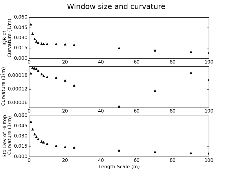
The plot is divided into three sections. The top plot is the change in the interquartile range of curvature with window size, the middle plot is the change in mean curvature with window size and the bottom plot is the change in the standard deviation of curvature with window size.

Roering et al. (2010) and Hurst et al. (2012) suggest that a clear scaling break can be observed in some or all of these three plots, which characterizes the transition from a length scale which captures meter-scale features such as tree throw mounds to a length scale which corresponds to individual hillslopes.

Care must be taken when using this technique as it is challenging to differentiate between measurement noise and topographic roughness (e.g. tree throw mounds) in data if the shot density of the point cloud from which the DEM is generated it too low or it has been poorly gridded. Pay close attention to the metadata provided with your topographic data. If none is provided this is probably a bad sign!

In our example, a length scale of between 4 and 8 meters would be appropriate, supported by the scaling breaks identified in the plots with the red arrows:

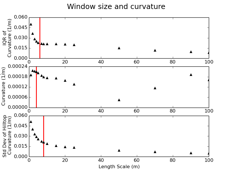
4. Legacy code: Extracting Hillslope Lengths

This section gives an overview of how to use the hillslope length driver (LH_Driver.cpp) and it’s companion (LH_Driver_RAW.cpp) to quickly generate hillslope length data for a series of basins, along with other basin average metrics within a larger DEM file.

For applications considering landscapes at geomorphic (millenial) timescales use the main driver, for event scale measurements use the RAW driver. All instructions on this page will work for either driver. For convenience it will refer only to LH_Driver.cpp but either driver can be used.

This code is used to to produce the data for Grieve et al. (in review.).

Quick guide if you already know what you are doing

Here is a quick overview of how to set up and run the code, if you have done it before:

Generate a channel head file for the landscape.
Get the window size for the surface fitting routines.
Compile the code with: make -f LH_Driver.make
Run the program LH_Driver.out using the path (with trailing slash), the filename prefix, window radius, basin order, a floodplain switch, and a switch to write rasters if desired as arguments.
Analyse the resulting data files using python.

4.1. Overview

This driver file will combine several LSDTopoTools Functions in order to generate as complete a range of basin average and hillslope length metrics as possible. The tool will generate:

A HilltopData file with metrics calculated for each hilltop pixel which can be routed to a stream pixel.
A file containing basin averaged values of hillslope lengths and other standard metrics.
An optional collection of trace files, which can be processed to create a shapefile of the trace paths across the landscape. These can be enabled by setting a flag inside the driver on line 141.

4.2. Input Data

This driver takes the following input data:

Table 12. Input data for the hillslope length code
Input data	Input type	Description
Raw DEM	A raster named `<prefix>_DEM.flt`.	The raw DEM to be analysed.
Channel Heads	Channel head raster named `<prefix>_DEM_CH.flt`.	A file containing channel heads, which can be generated using the DrEICH algorithm. See the [Channel extraction] chapter for more information.
Floodplain Mask	A binary mask of floodplains named `<prefix>_FloodPlain.flt`.	Floodplain data which can be used to ensure that analysis only occurs on the hillslopes. This is an optional input.
Surface Fitting Window Size	A float	The surface fitting window size can be constrained using the steps outlined in [Selecting A Window Size]. This should be performed to ensure the correct parameter values are selected.

4.3. Compile The Driver

The code is compiled using the provided makefile, LH_Driver.make and the command:

$ make -f LH_Driver.make

Which will create the binary file, LH_Driver.out to be executed.

4.4. Run The Hillslope Length Driver

The driver is run with six arguments:

Path

The data path where the channel head file and DEM is stored. The output data will be written here too.

Prefix

The filename prefix, without an underscore. If the DEM is called Oregon_DEM.flt the prefix would be Oregon. This will be used to give the output files a distinct identifier.

Window Size

Radius in spatial units of kernel used in surface fitting. Selected using window_size.

Stream Order

The Strahler number of basins to be extracted. Typically a value of 2 or 3 is used, to ensure a good balance between sampling density and basin area.

Floodplain Switch

If a floodplain raster has been generated it can be added to the channel network by setting this switch to 1. This will ensure that hillslope traces terminate at the hillslope-fluvial transition. If no floodplain raster is available, or required, this switch should be set to 0.

Write Rasters Switch

When running this driver several derivative rasters can be generated to explore the results spatially. If this is required, set this switch to 1. To avoid writing these files set the switch to 0. The rasters which will be written are:

A pit filled DEM
Slope
Aspect
Curvature
Stream network
Drainage basins of the user defined order
Hilltop curvature
Hillslope length
Hillslope gradient, computed as relief/hillslope length
Relief
A hillshade of the DEM

The syntax to run the driver on a unix machine is as follows:

$ ./LH_Driver.out <Path> <Prefix> <Window Radius> <Stream order> <Floodplain Switch> <Write Rasters Switch>

And a complete example (your path and filenames will vary):

$ ./LH_Driver.out /home/s0675405/DataStore/LH_tests/ Oregon 6 2 1 0

4.5. Analysing The Results

The final outputs are stored in two plain text files, which are written to the data folder supplied as the argument path.

4.5.1. <Prefix>_Paper_Data.txt

This file contains all of the basin average values for each basin, these files contain a large number of columns, providing a wealth of basin average data. The columns in the file, from left to right are as follows:

BasinID = Unique ID for the basin.
HFR_mean = Mean hilltop flow routing derived hillslope length.
HFR_median = Median hilltop flow routing derived hillslope length.
HFR_stddev = Standard deviation of hilltop flow routing derived hillslope length.
HFR_stderr = Standard error of hilltop flow routing derived hillslope length.
HFR_Nvalues = Number of values used in hilltop flow routing derived hillslope length.
HFR_range = Range of hilltop flow routing derived hillslope length.
HFR_min = Minimum hilltop flow routing derived hillslope length.
HFR_max = Maximum hilltop flow routing derived hillslope length.
SA_binned_LH = Hillslope length from binned slope area plot.
SA_Spline_LH = Hillslope length from spline curve in slope area plot.
LH_Density = Hillslope length from drainage density.
Area = Basin area.
Basin_Slope_mean = Mean basin slope.
Basin_Slope_median = Median basin slope.
Basin_Slope_stddev = Standard deviation of basin slope.
Basin_Slope_stderr = Standard error of basin slope.
Basin_Slope_Nvalues = Number of basin slope values.
Basin_Slope_range = Range of basin slopes.
Basin_Slope_min = Minimum basin slope.
Basin_Slope_max = Maximum basin slope.
Basin_elev_mean = Mean basin elevation.
Basin_elev_median = Median basin elevation.
Basin_elev_stddev = Standard deviation of basin elevation.
Basin_elev_stderr = Standard error of basin elevation.
Basin_elev_Nvalues = Number of basin elevation values.
Basin_elev_Range = Range of basin elevations.
Basin_elev_min = Minimum basin elevation.
Basin_elev_max = Maximum basin elevation.
Aspect_mean = Mean aspect of the basin.
CHT_mean = Mean hilltop curvature of the basin.
CHT_median = Median hilltop curvature of the basin.
CHT_stddev = Standard deviation of hilltop curvature of the basin.
CHT_stderr = Standard error of hilltop curvature of the basin.
CHT_Nvalues = Number of hilltop curvature values used.
CHT_range = Range of hilltop curvatures.
CHT_min = Minimum hilltop curvature in the basin.
CHT_max = Maximum hilltop curvature in the basin.
EStar = \(E*\) value from Roering et al. (2007).
RStar = \(R*\) value from Roering et al. (2007).
HT_Slope_mean = Mean slope calculated using (relief/hillslope length).
HT_Slope_median = Median slope calculated using (relief/hillslope length).
HT_Slope_stddev = Standard deviation of slope calculated using (relief/hillslope length).
HT_Slope_stderr = Standard error of slope calculated using (relief/hillslope length).
HT_Slope_Nvalues = Number of slope values calculated using (relief/hillslope length).
HT_Slope_range = Range of slopes calculated using (relief/hillslope length).
HT_Slope_min = Minimum slope calculated using (relief/hillslope length).
HT_Slope_max = Maximum slope calculated using (relief/hillslope length).
HT_relief_mean = Mean relief.
HT_relief_median = Median relief.
HT_relief_stddev = Standard deviation of relief.
HT_relief_stderr = Standard error of relief.
HT_relief_Nvalues = Number of relief values used.
HT_relief_range = Range of reliefs.
HT_relief_min = Minimum relief.
HT_relief_max = Maximum relief.

This file can be loaded and the data visualized using these python scripts.

4.5.2. <Prefix>_HilltopData.csv

This file contains hillslope metrics calculated for every hilltop pixel in the dataset which was routed successfully to a stream pixel. The columns in the file, from left to right are as follows:

X is the x coordinate of the hilltop pixel.
Y is the x coordinate of the hilltop pixel.
hilltop_id is the value of the hilltop pixel.
S is the slope calculated as relief/hillslope length.
R is the relief, the change in elevation between the hilltop and the channel
Lh is the hillslope flow length.
BasinID is the junction outlet number of the basin the hilltop is within.
StreamID is the value of the stream pixel reached by the trace.
HilltopSlope is the gradient of the pixel hwere the trace started.
DivergentCountFlag is the count of divergent pixels crossed. Depreciated
PlanarCountFlag - Count of planar cells crossed Depreciated
E_Star = \(E*\) value from Roering et al. (2007).
R_Star = \(R*\) value from Roering et al. (2007).
EucDist - Euclidean length of the trace from hilltop to channel

This file can be loaded and the data visualized using these python scripts.

4.5.3. Trace Files

An optional switch can be set within the code to print out the coordinates of the path of each trace, allowing hilltop flow paths to be visualized. This option is not exposed at the command line as it will considerably slow the execution of the algorithm.

This will generate a large number of text files, which some operating systems can struggle to handle.

To enable this feature open the driver file LH_Driver.cpp and find the following parameters which should be located around line 140:

bool print_paths_switch = false;
int thinning = 1;
string trace_path = "";
bool basin_filter_switch = false;
vector<int> Target_Basin_Vector;

These control the path file printing and give several options to limit the scope of the path printing to ensure a manageable number of files are generated. The possible values for each parameter are:

Table 13. Path file printing parameters
Parameter	Input type	Description
`print_paths_switch`	bool	Set this to `true` to print paths and `false` to not print paths (the default)
`thinning`	int	The default value of `1` will keep every trace, whereas any other value will thin the data and write every `nth` trace to a file.
`trace_path`	string	The directory that the trace files will be written to, it is strongly recommended that this be an empty directory.
`basin_filter_switch`	bool	Set this to `true` if you only want to write trace files contained within traget basins. `false` will process the whole DEM.
`Target_Basin_Vector`	Vector of ints	If `basin_filter_switch` is set to true, populate this vector with the IDs of the basins to be studied.

Once these parameters have been set, re-compile the driver following the steps in Compile The Driver and run the code. Once the code has executed a large number of files will have been generated in the supplied path. They are plain text, space delimited files which have the following headings:

X Coordinate.
Y Coordinate.
Count of divergent pixels crossed during the trace.
Hillslope length.
Count of planar pixels crossed during the trace.
E_Star from Roering et al. (2007).
R_Star from Roering et al. (2007).
Euclidean length of trace.

A python script is provided to process these files into a shapefile, which can be viewed in any GIS package, or plotted using other python scripts provided. The python script to process these files is located here and is called trace_process_1_1.py. To run this file, alter the input path to point to where the trace files are stored, and then set the output path to a new directory which must already exist.

The line:

files = files[::100] # only processing every 100th trace for speed

is used to thin the dataset to speed up processing, in case this was not performed earlier. Again, a value of 1 will keep all of the data, and any other integer will keep every nth file. Once the code has been executed a single shapefile will be produced in the user defined output directory.

4.6. Worked Example

In this final section a typical hillslope length analysis will be performed from start to finish to demonstrate how to use this algorithm on real data. For this example we will use a very small section of Gabilan Mesa, to facilitate rapid processing.

4.6.1. Getting the data

The data is located in the ExampleTopoDatasets repository. Firstly, we must create a new directory to store our topogrpahic data:

$ mkdir data
$ pwd
/home/s0675405/LH/data/

We will only take the data we need, which is the Gabilan Mesa DEM and the associated DrEICH channel head file, so we can use wget to download the data:

$ wget https://github.com/LSDtopotools/ExampleTopoDatasets/raw/master/gabilan.bil
$ wget https://github.com/LSDtopotools/ExampleTopoDatasets/raw/master/gabilan.hdr
$ wget https://github.com/LSDtopotools/ExampleTopoDatasets/raw/master/gabilan_CH.bil
$ wget https://github.com/LSDtopotools/ExampleTopoDatasets/raw/master/gabilan_CH.hdr

You should now have the following files in your data folder:

$ pwd
/home/s0675405/LH/data/
$ ls
gabilan.bil  gabilan_CH.bil  gabilan_CH.hdr  gabilan.hdr

4.6.2. Getting The Code

Next we need to download the code from the CSDMS repository where the latest stable version of the hilltop flow routing algorithm is located. This can again be downloaded using wget and it will come as a zipfile, which should be extracted into a separate folder to the data:

$ wget https://github.com/csdms-contrib/Hilltop_flow_routing/archive/master.zip
$ unzip master.zip

Finally we need to get the visualization python scripts so we can explore the data:

$ wget https://github.com/sgrieve/LH_Paper_Plotting/archive/master.zip
$ unzip master.zip

Now we should have 3 folders, one with the data, one with the main c++ code and a third with the python code.

$ ls
data  Hilltop_flow_routing-master  LH_Paper_Plotting-master

4.6.3. Running The Code

We need to check that the filenames for our input and output data make sense in the LH_Driver.cpp file. Open the file in a text editor and look at the line which loads the DEM:

LSDRaster DEM((path+filename+"_dem"), "flt");

We are working with bil files, so need to change the "flt" to "bil", which can be done with a simple search and replace within your text editor.

The code also expects our data to be tagged *_dem so lets rename our data files to make life simpler:

$ pwd
/home/s0675405/LH/data
$ mv gabilan.bil gabilan_dem.bil
$ mv gabilan.hdr gabilan_dem.hdr
$ mv gabilan_CH.bil gabilan_dem_CH.bil
$ mv gabilan_CH.hdr gabilan_dem_CH.hdr
$ ls
gabilan_dem.bil  gabilan_dem_CH.bil  gabilan_dem_CH.hdr  gabilan_dem.hdr

Now we can navigate back to the directory where the driver and makefile are stored and make the driver:

$ pwd
/home/s0675405/LH/Hilltop_flow_routing-master/driver_functions_GrieveLH2015
$ make -f LH_Driver.make
g++ -c -Wall -O3 -pg -g ../LSDParticle.cpp -o ../LSDParticle.o
g++ -c -Wall -O3 -pg -g ../LSDCRNParameters.cpp -o ../LSDCRNParameters.o
g++ -Wall -O3 -pg -g LH_Driver.o ../LSDMostLikelyPartitionsFinder.o ../LSDIndexRaster.o ../LSDRaster.o ../LSDFlowInfo.o ../LSDJunctionNetwork.o ../LSDIndexChannel.o ../LSDChannel.o ../LSDStatsTools.o ../LSDBasin.o ../LSDShapeTools.o ../LSDParticle.o ../LSDCRNParameters.o -o LH_Driver.out

Some warnings may appear which can be ignored as long as the final few lines look something like they do above and the file LH_Driver.out is created.

The binary file can then be run using the desired input arguments

./LH_Driver.out /home/s0675405/LH/data/ gabilan 5 2 0 0

Once the code is completed it will print some data to the screen about the success rate of the traces. Due to the nature of real topography there will always be a small number of failed traces, traces which hit the edge of the DEM should also be rare, but these are excluded from analysis as they are truncated. If these values are very large relative to the stream count, which denotes traces which have successfully completed, there may be a problem with your input data. In the case of this worked example we get the following results:

Hilltop count: 2170
Stream count: 2157
Fail count: 7
Uphill count: 0
Edge count: 6

Returning to the data folder we can see the the two data files described earlier in this chapter have been written.

$ pwd
/home/s0675405/LH/data
$ ls
gabilan_dem.bil     gabilan_dem_CH.hdr  gabilan_dreich__HilltopData.csv
gabilan_dem_CH.bil  gabilan_dem.hdr     gabilan_dreich_PaperData.txt

4.6.4. Plotting Data

We can now load the data files into the python scripts to visualize the data. Firstly, we can make a histogram to view the distribution of hillslope length values for our landscape using the RAW_LH_Hist.py script. We need to update the plotting parameters to reflect our data, the following lines can be edited within the script using any text editor:

#================ modifyable parameters start here ====================

#paths to the data and to save the figure to
path = '../../data/' #path to the folder contaning the hilltopdata files
filename = 'gabilan_dreich__HilltopData.csv'
figpath = path #path to save the final figures

#plot style parameters
xmax = 400
ymax = 40
xstep = 50
ystep = 10
title_move = 0.

#plot labels
location = 'Gabilan Mesa'

#================ modifyable parameters end here ====================

The plot style parameters require a bit of trial and error to get the the correct axis limits, so the code may need to be executed several times. Once the parameters have been set the script can be run at the command line:

python RAW_LH_Hist.py

Which produces a histogram within the data folder.

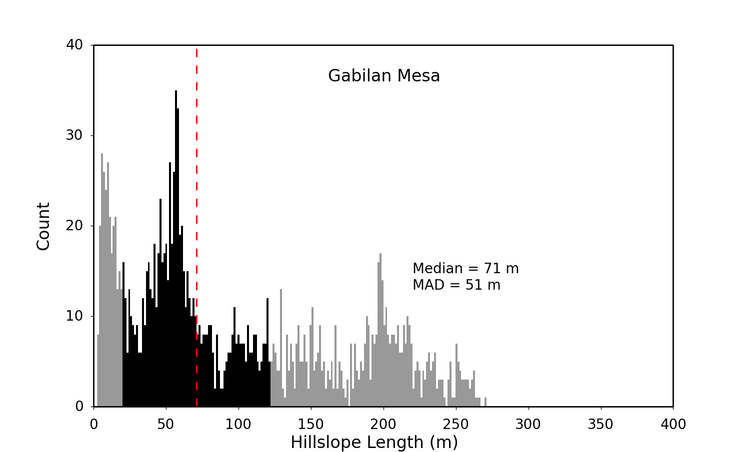
This process can be repeated to run any of the plotting scripts provided with this package, as each has a similar interface.

4.7. Summary

You should now be able to generate hillslope length data from high resolution topography.

5. Legacy code: Dimensionless Erosion and Relief

The relationship between topographic relief and erosion rate can be used to interrogate dynamic forces which interact to shape the Earth’s surface. Roering et al. (2007) formulated a dimensionless relationship between relief (R*) and erosion rate (E*) which allows comparisons between landscapes of vastly differing forms. Hurst et al. (2013) used this technique to identify topographic uplift and decay along the Dragons Back Pressure Ridge, CA. However, in spite of its utility, it has always been a challenging method to implement. In this chapter we go through the steps required to generate E* R* data using LSDTopoTools from high resolution topography at a range of spatial scales, following Grieve et al. (2015).

Quick guide if you already know what you are doing

Here is a quick overview of how to set up and run the code, if you have done it before:

Generate a channel head file for the landscape.
Run the hillslope lenth driver, following the [Extracting Hillslope Lengths] chapter.
Compile the code with: make -f E_STAR_R_STAR.make
Run the program E_STAR_R_STAR.out using the path (with trailing slash), the filename prefix, the minimum patch area in pixels, the minimum number of data points per basin and the basin order.
Analyze the resulting data files using Plot_ER_Data.py.

5.1. Get the code for dimensionless erosion and relief analysis

Our code for E*R* analysis can be found in our GitHub repository. This repository contains code for extracting channel networks, generating hillslope length data and processing this topographic data into a form which can be used to generate E* R* relationships.

5.1.1. Clone the GitHub repository

First navigate to the folder where you will keep the GitHub repository. In this example it is called /home/LSDTT_repositories. To navigate to this folder in a UNIX terminal use the cd command:

$ cd /home/LSDTT_repositories/

You can use the command pwd to check you are in the right folder. Once you are in this folder, you can clone the repository from the GitHub website:

$ pwd
/home/LSDTT_repositories/
$ git clone https://github.com/LSDtopotools/LSDTT_Hillslope_Analysis.git

Navigate to this folder again using the cd command:

$ cd LSDTT_Hillslope_Analysis/

5.1.2. Alternatively, get the zipped code

If you don’t want to use git, you can download a zipped version of the code:

$ pwd
/home/LSDTT_repositories/
$ wget https://github.com/LSDtopotools/LSDTT_Hillslope_Analysis/archive/master.zip
$ gunzip master.zip

GitHub zips all repositories into a file called master.zip, so if you previously downloaded a zipper repository this will overwrite it.

5.1.3. Get the Python code

In addition to the topographic analysis code, some python code is provided to handle the generation of the E* R* data and its visualization. This code is stored in a separate GitHub repository which can be checked out in the same manner as before. It is a good idea to place the python code into a separate directory to avoid confusion later on.

$ pwd
/home/LSDTT_repositories/
$ git clone https://github.com/sgrieve/ER_Star.git

Navigate to this folder again using the cd command:

$ cd ER_STAR/

or if you prefer to avoid git:

$ pwd
/home/LSDTT_repositories/
$ wget https://github.com/LSDtopotools/LSDTopoTools_ER_STAR/archive/master.zip
$ gunzip master.zip

The python code has a number of dependences which you should check prior to trying to run the code, as it could give confusing error messages.

5.1.4. Checking your Python package versions

For the code to run correctly the following packages must be installed with a version number greater than or equal to the version number listed below. The code has only been tested on Python 2.7 using the listed versions of these packages, so if you experience unexpected behavior on a higher version, try installing the specified version.

matplotlib: Version 1.43
numpy: Verision 1.9.2
scipy: Version 0.16.0
uncertainties: Version 2.4.6

To test if you have a package installed, launch python at the terminal and try to import each package in turn. For example, to test if we have numpy installed:

$ python
Python 2.7.6 (default, Jun 22 2015, 18:00:18)
[GCC 4.8.2] on linux2
Type "help", "copyright", "credits" or "license" for more information.
>>> import numpy
>>>

If importing the package does nothing, that means it has worked, and we can now check the version of numpy

>>> numpy.__version__
>>> '1.9.2'

In this case my version of numpy is new enough to run Plot_ER_Data.py without any problems. Repeat this test for each of the 4 packages and if any of them are not installed or are too old a version, it can be installed by using pip at the unix terminal or upgraded by using the --upgrade switch.

$ sudo pip install <package name>
$ sudo pip install --upgrade <package name>

5.1.5. Get the example datasets

We have provided some example datasets which you can use in order to test this algorithm. In this tutorial we will work using a LiDAR dataset and accompanying channel heads from Gabilan Mesa, California. You can get it from our ExampleTopoDatasets repository using wget and we will store the files in a folder called data:

$ pwd
/home/data
$ wget https://github.com/LSDtopotools/ExampleTopoDatasets/raw/master/gabilan.bil
$ wget https://github.com/LSDtopotools/ExampleTopoDatasets/raw/master/gabilan.hdr
$ wget https://github.com/LSDtopotools/ExampleTopoDatasets/raw/master/gabilan_CH.bil
$ wget https://github.com/LSDtopotools/ExampleTopoDatasets/raw/master/gabilan_CH.hdr

This dataset is already in the preferred format for use with LSDTopoTools (the ENVI bil format). However the filenames are not structured in a manner which the code expects. Both the hillslope length driver and the E*R* driver expect files to follow the format <prefix>_<filetype>.bil so we should rename these four files to follow this format.

$ pwd
/home/so675405/data
$ mv gabilan.bil gabilan_DEM.bil
$ mv gabilan.hdr gabilan_DEM.hdr
$ mv gabilan_CH.bil gabilan_DEM_CH.bil
$ mv gabilan_CH.hdr gabilan_DEM_CH.hdr
$ ls
gabilan_DEM.bil  gabilan_DEM_CH.bil  gabilan_DEM_CH.hdr  gabilan_DEM.hdr

Now the prefix for our data is gabilan and we are ready to look at the code itself.

5.2. Processing High Resolution Topography

The generation of E* R* data is built upon the ability to measure hillslope length and relief as spatially continuous variables across a landscape. This is performed by using the hillslope length driver outlined in the [Extracting Hillslope Lengths] chapter.

When running the hillslope length driver, ensure that the switch to write the rasters is set to 1 as these rasters are required by the E_STAR_R_STAR.cpp driver.

This driver performs the hilltop segmentation and data averaging needed to generate E* R* data at the scale of individual hilltop pixels, averaged at the hillslope scale and at a basin average scale.

5.3. Input Data

This driver takes the following input data:

Table 14. Input data for the `E_STAR_R_STAR.cpp` driver.
Input data	Input type	Description
Raw DEM	A raster named `<prefix>_DEM.flt`.	The raw DEM to be analysed.
Hillslope length raster	A raster named `<prefix>_HFR_LH.flt`.	A raster of hillslope length measurements generated by `LH_Driver.cpp`.
Topographic relief raster	A raster named `<prefix>_Relief.flt`.	A raster of topographic relief measurements generated by `LH_Driver.cpp`.
Hilltop curvature raster	A raster named `<prefix>_CHT.flt`.	A raster of hilltop curvature measurements generated by `LH_Driver.cpp`.
Slope raster	A raster named `<prefix>_Slope.flt`.	A raster of topographic gradient generated by `LH_Driver.cpp`.
Minimum Patch Area	An integer	The minimum number of pixels required for a hilltop to be used for spatial averaging.
Minimum Number of Basin Data Points	An integer	The minimum number of data points required for each basin average value to be computed.
Basin Order	An integer	The Strahler number of basins to be extracted. Typically a value of 2 or 3 is used, to ensure a good balance between sampling density and basin area.

5.4. Compile The Driver

Once you have generated the hillslope length data you must compile the E_STAR_R_STAR.cpp driver. This is performed by using the provided makefile, LH_Driver.make and the command:

$ make -f E_STAR_R_STAR.make

Which will create the binary file, E_STAR_R_STAR.out to be executed.

5.5. Run the code

Once the driver has been compiled it can be run using the following arguments:

Path: The data path where the input data files are stored. The output data will be written here too.
Prefix: The filename prefix, without an underscore. If the DEM is called Oregon_DEM.flt the prefix would be Oregon. This will be used to give the output files a distinct identifier.
Minimum Patch Area: The minimum number of pixels required for a hilltop to be used for spatial averaging.
Minimum Number of Basin Data Points: The minimum number of data points required for each basin average value to be computed.
Basin Order: The Strahler number of basins to be extracted. Typically a value of 2 or 3 is used, to ensure a good balance between sampling density and basin area.

In our example we must navigate to the directory where the file was compiled and run the code, providing the five input arguments:

$ pwd
/home/LSDTT_repositories/ER_Code_Package/Drivers
$ ./E_STAR_R_STAR.out /home/data/ gabilan 50 50 2

A more general example of the input arguments would is:

$ ./E_STAR_R_STAR.out <path to data files> <filename prefix> <min. patch area> <min. basin pixels> <basin order>

Once the code has run, it will produce 5 output files, tagged with the input filename prefix. In the case of our example, these files are:

gabilan_E_R_Star_Raw_Data.csv
gabilan_E_R_Star_Patch_Data.csv
gabilan_E_R_Star_Basin_2_Data.csv
gabilan_Patches_CC.bil
gabilan_Patches_CC.hdr

The three .csv files are the data files containing the raw, hilltop patch and basin average data which is used by Plot_ER_Data.py to generate the E* R* results. The .bil and accompanying .hdr files contain the hilltop network used for the spatial averaging of the data, with each hilltop coded with a unique ID. This can be used to check the spatial distribution of hilltops across the study site.

5.6. Analyzing Dimensionless Relationships

Once the code has been run and the data has been generated, it can be processed using the Python script Plot_ER_Data.py which was downloaded into the directory:

$ pwd
/home/LSDTT_repositories/ER_Star
$ ls
bin_data.py  Plot_ER_Data.py  Settings.py

The three Python files are all needed to perform the E* R* analysis. The main code is contained within Plot_ER_Data.py and it makes use of bin_data.py to perform the binning of the data. The file Settings.py is the file that users should modify to run the code on their data.

Settings.py is a large parameter file which must be modified to reflect our input data and the nature of the plots we want to generate. Each parameter is described within the file, but these descriptions are also produced here for clarity. It should be noted that a useful method for managing large sets of data and plotting permutations is to generate several Settings.py files and swapping between them as needed. The following tables outline all of the parameters which can be used to configure the E* R* plots.

Table 15. Paramter information to load data.
Parameter Name	Possible Values	Description
Path	Any valid path	Must be wrapped in quotes with a trailing slash eg 'home/user/data/'
Prefix	Filename prefix	Must be wrapped in quotes and match the prefix used in `ER_STAR.cpp`
Order	Any integer	Basin order used in `ER_STAR.cpp` to extract the drainage basins. eg 1,2,5

Table 16. Options to select data to be plotted
Parameter Name	Possible Values	Description
RawFlag	0 or 1	Use 1 to plot the raw data and 0 to not plot it.
DensityFlag	Any integer	Use 0 to not plot the raw data as a density plot and 1 to plot a density plot. Values greater than 1 will be used the thin the data. For example 2 will plot every second point. Reccommended!
BinFlag	'raw', 'patches' or ''	Use 'raw' to bin the raw data, 'patches' to bin the hilltop patch data and an empty string, '' to not perform binning. Note that quotes are needed for all cases.
NumBins	Any integer	Number of bins to be generated. Must be an integer. eg 5,11,20. Will be ignored if `BinFlag` is left blank.
MinBinSize	Any integer	Minimum number of data points required for a bin to be valid. eg 5,20,100. Will be ignored if `BinFlag` is left blank.
PatchFlag	0 or 1	Use 1 to plot the patch data and 0 to not plot it.
BasinFlag	0 or 1	Use 1 to plot the basin data and 0 to not plot it.
LandscapeFlag	0 or 1	Use 1 to plot the landscape average data and 0 to not plot it.

Table 17. Options controlling the fitting of the critical gradient
Parameter Name	Possible Values	Description
Sc_Method	A real number or 'raw', 'patches' or 'basins'	Either input a real number eg 0.8,1.2,1.052 to set the Sc value and avoid the fitting of Sc. Or select 'raw','patches' or 'basins' (including the quotes) to use the named dataset to constrain the best fit Sc value through bootstrapping.
NumBootsraps	Any integer	Number of iterations for the bootstrapping procedure. 10000 is the default, larger values will take longer to process.

Table 18. Options controlling the plot style
Parameter Name	Possible Values	Description
ErrorBarFlag	True or False	True to plot errorbars on datapoints, False to exclude them. Errorbars are generated as the standard error unless otherwise stated.
Format	'png','pdf','ps','eps','svg'	File format for the output E* R* plots. Must be one of: 'png','pdf','ps','eps','svg', including the quotes.
GabilanMesa	True or False	True to plot the example data from Roering et al. (2007), False to exclude it.
OregonCoastRange	True or False	True to plot the example data from Roering et al. (2007), False to exclude it.
SierraNevada	True or False	True to plot the example data from Hurst et al. (2012), False to exclude it.

5.6.1. Density Plot

Firstly we will generate a density plot from the raw E* R* data. To do this we must update the path to our data files, the prefix and the basin order so that our files can be loaded. These modifications can be done in any text editor.

As we want to display a density plot we must also place a value other than 0 for the DensityFlag parameter, and ensure that all other parameters in the second parameter table are set to 0 or in the case of BinFlag, an empty string ''.

We will set the critical gradient to a value of 0.8, to avoid running the bootstrapping calculations. ErrorBarFlag should be set to False, along with the example data options, and the file format can be left as the default value.

The below complete settings file has the comments removed for clarity, as these are not needed by the program.

# Parameters to load the data
Path = '/home/s0675405/data/'
Prefix = 'gabilan'
Order = 2

# Options to select data to be plotted
RawFlag = 0
DensityFlag = 1
BinFlag = ''
NumBins = 20
MinBinSize = 100
PatchFlag = 0
BasinFlag = 0
LandscapeFlag = 0

# Options regarding the fitting of the critical gradient
Sc_Method = 0.8
NumBootsraps = 100

# Plot style options
ErrorBarFlag = False
Format = 'png'

# Comparison data to be plotted from the other studies
GabilanMesa = False
OregonCoastRange = False
SierraNevada = False

Once the settings file has been generated, the code can be run from the terminal:

$ python Plot_ER_Data.py

This will write a file called gabilan_E_R_Star.png to the data folder, which should look like this:

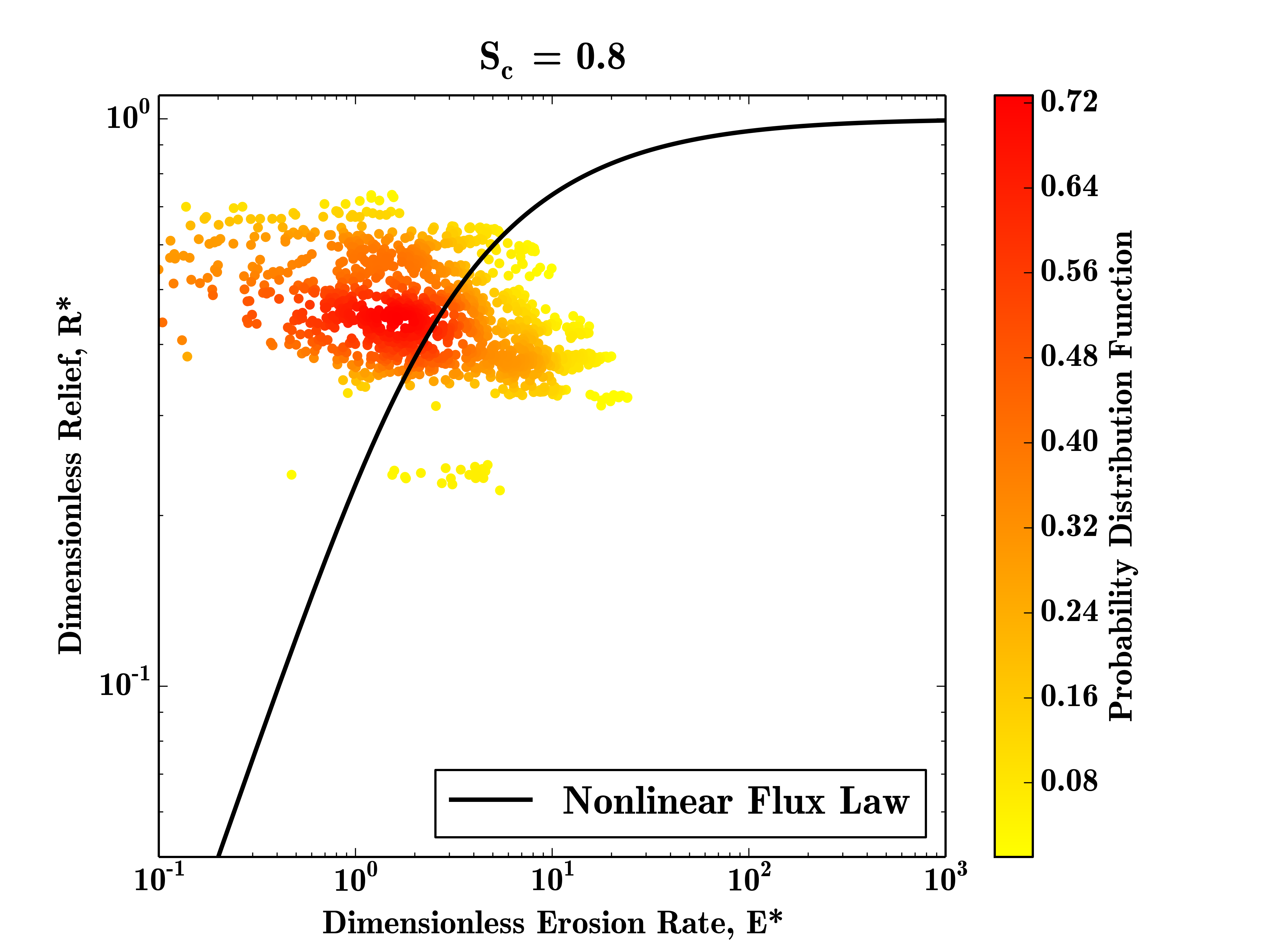
This plot shows the density of the E* R* measurements for this test datatset, the data is quite sparse due to the small size of the input DEM, but the majority of data points still plot close to the steady state curve.

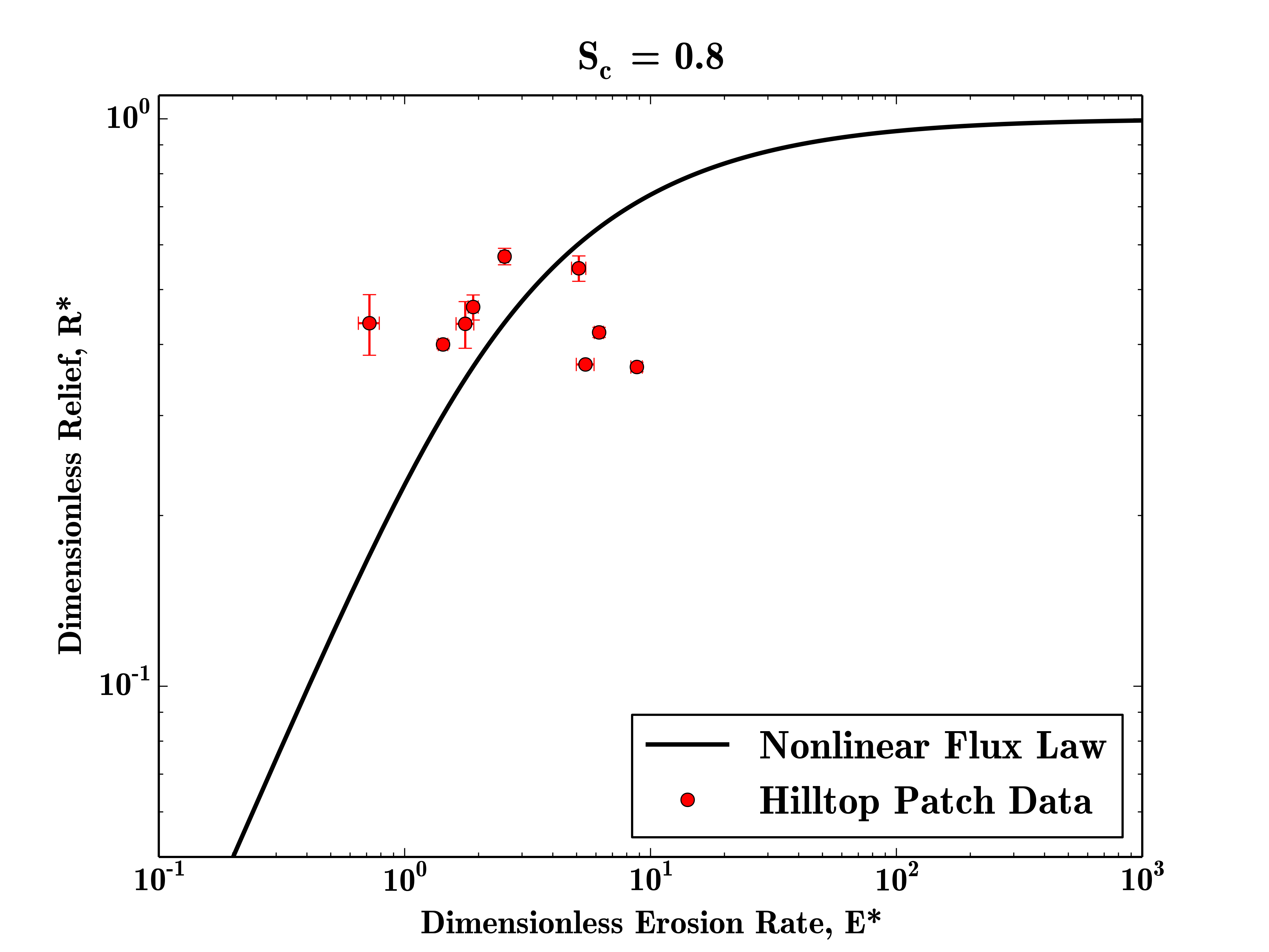
5.6.2. Hilltop Patch Plot

Having completed the first example plot it becomes very simple to re-run the code to generate different plots. In this example we will plot the hilltop patch data points with error bars. To do this we need to change our settings file as follows:

# Parameters to load the data
Path = '/home/s0675405/data/'
Prefix = 'gabilan'
Order = 2

# Options to select data to be plotted
RawFlag = 0
DensityFlag = 0
BinFlag = ''
NumBins = 20
MinBinSize = 100
PatchFlag = 1
BasinFlag = 0
LandscapeFlag = 0

# Options regarding the fitting of the critical gradient
Sc_Method = 0.8
NumBootsraps = 100

# Plot style options
ErrorBarFlag = True
Format = 'png'

# Comparison data to be plotted from the other studies
GabilanMesa = False
OregonCoastRange = False
SierraNevada = False

This set of parameters generates a small number of hilltop patch data points which plot in similar locations as the raw data.

To plot the basin average data, the same set of paramters would be used

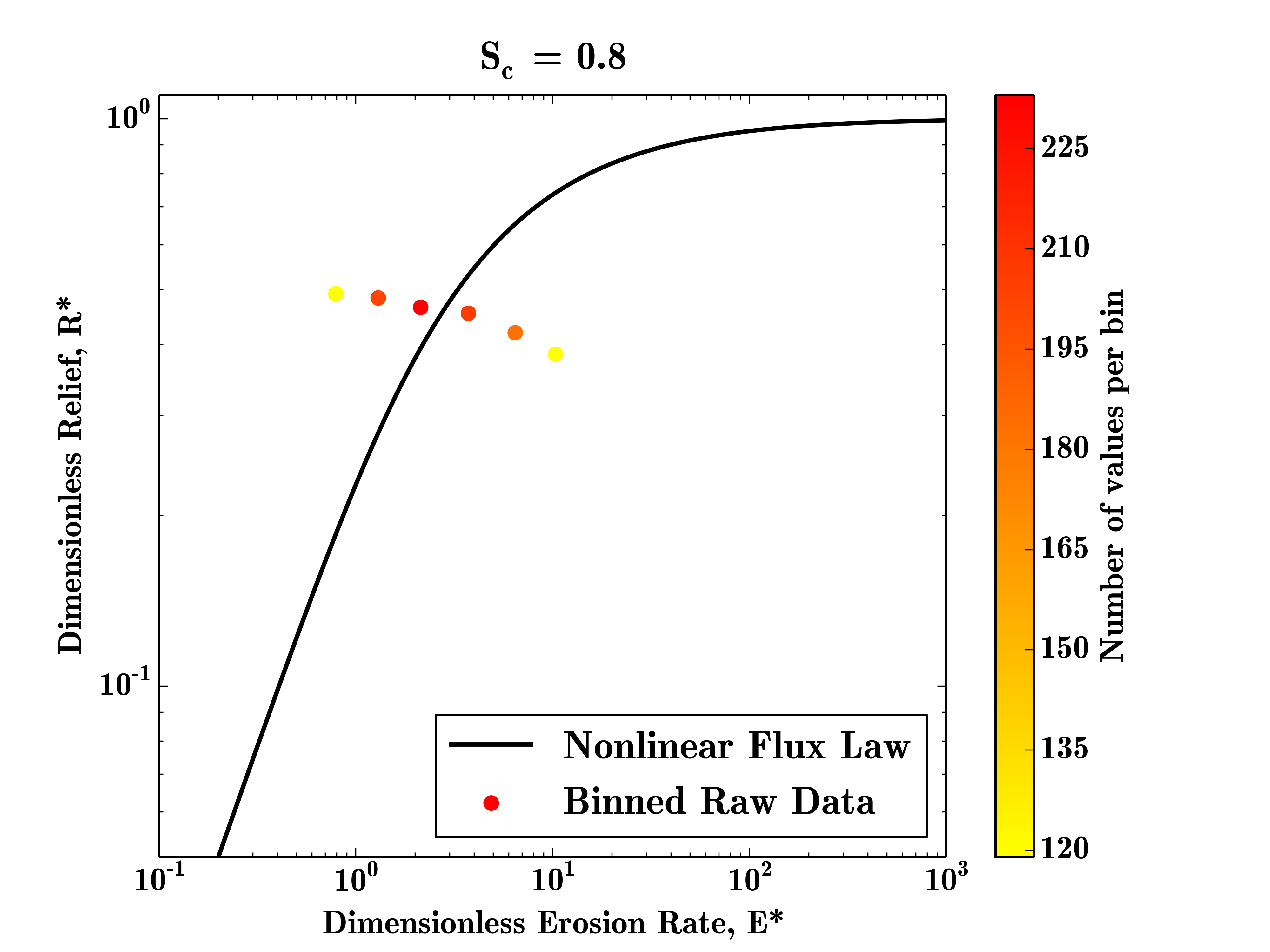
5.6.3. Binned Plot

To bin the raw data, we need to set the BinFlag parameter to 'raw' and select a number of bins to place our data into:

# Parameters to load the data
Path = '/home/s0675405/data/'
Prefix = 'gabilan'
Order = 2

# Options to select data to be plotted
RawFlag = 0
DensityFlag = 0
BinFlag = 'raw'
NumBins = 20
MinBinSize = 100
PatchFlag = 0
BasinFlag = 0
LandscapeFlag = 0

# Options regarding the fitting of the critical gradient
Sc_Method = 0.8
NumBootsraps = 100

# Plot style options
ErrorBarFlag = True
Format = 'png'

# Comparison data to be plotted from the other studies
GabilanMesa = False
OregonCoastRange = False
SierraNevada = False

In this case, the result is fairly meaningless, as most of the bins have too few data points to be plottted, but on larger datasets this method can highlight landscape transience very clearly.

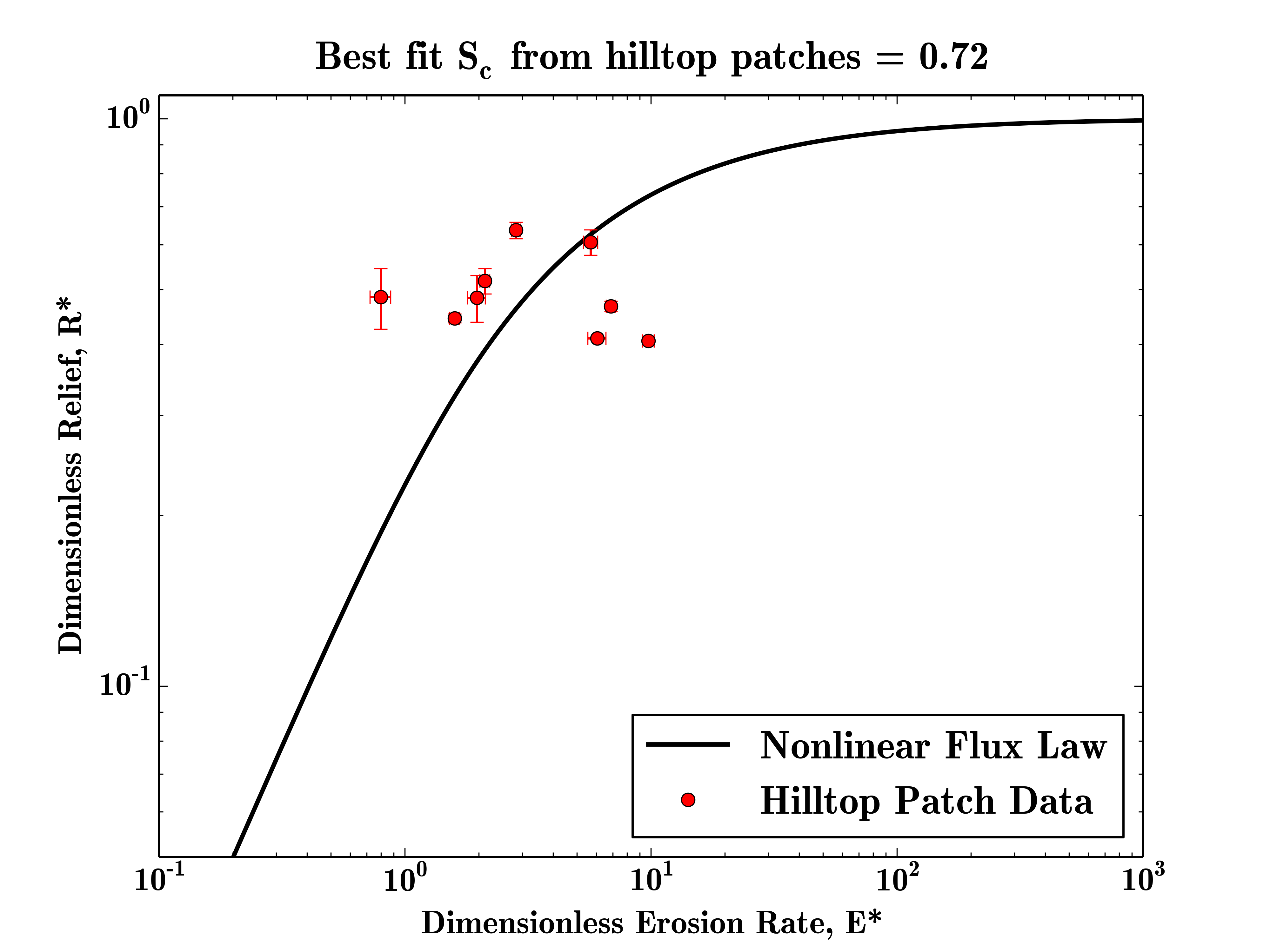
5.6.4. Fitting The Critical Gradient

The final example for this section is how to use the code to estimate the critical gradient of a landscape. This is performed by configuring the bootstrapping parameters and in this case we will use the patch data and 1000 iterations to compute the best fit critical gradient.

# Parameters to load the data
Path = '/home/s0675405/data/'
Prefix = 'gabilan'
Order = 2

# Options to select data to be plotted
RawFlag = 0
DensityFlag = 0
BinFlag = ''
NumBins = 20
MinBinSize = 100
PatchFlag = 1
BasinFlag = 0
LandscapeFlag = 0

# Options regarding the fitting of the critical gradient
Sc_Method = 'patches'
NumBootsraps = 1000

# Plot style options
ErrorBarFlag = True
Format = 'png'

# Comparison data to be plotted from the other studies
GabilanMesa = False
OregonCoastRange = False
SierraNevada = False

It should be noted that on a small dataset such as this the fitting will not be very robust as there are too few data points, but this example should demonstrate how to run the code in this manner on real data. The best fit critical gradient will be printed at the top of the final plot.

5.7. Summary

By now you should be able to generate dimensionless erosion rate and relief data from high resolution topography.