A reminder for DAV

I had a weird bug the other day that was caused by mixing up the behaviour of std::vector and the TNT::Array types. The C++ vector from the Standard Template Library has default initialisation values for certain built in types like int, float, double etc. So if you create a std::vector like this:

std::vector<double> MyVec(10);

It will have ten elements, all of type double, and they will be default initiaised to 0. Same is true for ints and floats. Strings receive an empty string: "". You can also specify another initialisation value if you don’t want the deafult.

std::vector<int> MyVecInts(10, 42);   // 10 ints all of value 42

But the TNT::Array type used in LSDTopoTools doesn’t do this for you. If you don’t initialise the array, it will contain garbage values from whatever happens to be in memory:

TNT::Array2D<double> MyArray(100, 100);     // 100 x 100 array, no initialisation.

Instead I should have specified the initialisation value, like:

TNT::Array2D<double> MyArray(100, 100, 0.0)     // 100 x 100 array, all zeros

Or initialised it with a for loop, or some other method.

In a previous post, I did a rough, back-of-the-envelope scaling benchmark with some flooding simulations running on a multicore compute-node, including some simulations on my desktop PC. I’ve revisited this to make the scaling comparisons at bit more consistent (sticking to the compute node CPUs on ARCHER, rather than mixing and matching different hardware). There’s also a nice scaling graph, so everyone’s happy. Gotta love a good scaling graph.

The simulation is run with the Boscastle catchment in Cornwall, simulating a flood event over 48 hours. (The devastating flood of 2004.) Two sets of simulations are done, one running as a hydrological model only, and the other with erosion and sediment transport switched on, which is generally a bit mode computationally expensive.

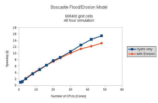
As a lot of the code has sections that have to be done serially, there’s not a 1:1 scaling of CPUs to speed-up-multiplier, which is to be expected. But I’m quite happy with this for now; if I’ve got time at some point, I’ll delve into OpenMP some more and look for other areas of the code to parallelise. Obviously the simulations with the erosion routines switched on take a lot longer to do: They don’t parallelise quite so well, and there’s a lot more computation with all the different grain sizes etc. While the hydro model speed up is roughly linear all the way up to around 48 cores (you can just see it tailing off perhaps around 40 cores…) the erosion simulations speed-up clearly starts to tail off around 24 cores upwards.

The actual run times can be compared with the graph below:

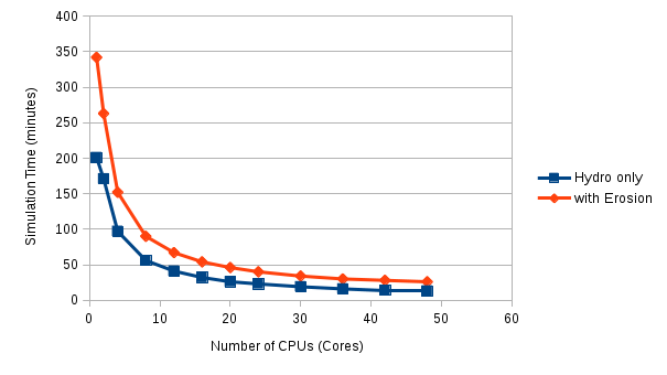
Actual run times with erosion routines on are approaching double that with just the hydrological model, in serial. However as both codes scale up over more CPUs, the gap narrows, relatively speaking. All these simulations are run with around 600000 grid cells (a 5m resolution DEM). Future work will look at some larger model domains to see how this affects scaling. (Spoiler alert: guess what, it does!)

No. You cannot strictly speaking, overload Python functions. One reason being is that types are not specified in function definitions (the language is Dynamically Typed anyway, and accepts optional function arguments.)

If you want different function behaviour based on different types, you have to introduce some conditional logic. I wanted to ‘overload’ this function so it was either supplied a filepath to a raster, which it then converted to an array, or would be supplied a NumPy array directly:

def DrapedOverHillshade(FileName, DrapeName, thiscmap='gray',drape_cmap='gray',
                            colorbarlabel='Elevation in meters',clim_val = (0,0),
                            drape_alpha = 0.6, ShowColorbar = False):
                            

So DrapeName could either be type numpy.ndarray or str. At the appropriate point in the function, I added a check to find what type had actually been passed, then called a relevant function if a file -> array conversion was needed.

if isinstance(DrapeName, str):
  raster_drape = LSDMap_IO.ReadRasterArrayBlocks(DrapeName)
elif isinstance(DrapeName, np.ndarray):
  raster_drape = DrapeName
else:
  print "DrapeName supplied is of type: ", type(DrapeName)
  raise ValueError('DrapeName must either be a string to a filename, \
  or a numpy ndarray type. Please try again.')

Not this uses isinstance(object, type) rather than something which might be more intuitive like if type(DrapeName) is type for example. This is because type() only checks for the exact type specified - and would ignore any subtype or subclass of the object specified.

It would also have been possible to not check the type at all, and just use a try, catch statement, first treating DrapeArray as a string, then as an array. (And actually, some people might consider this to be the more pythonic way of doing it…)

In an earlier post, I looked at how the LSDCatchmentModel scaled up to running on a single cluster-computer compute-node. The example ran tests on a small catchment in hydrological mode only (i.e. no erosion modules turned on). The algorithm for water routing used in the model (Bates et al., 2010), had already been well investigated and tested in other parallel implementations, showing a favourable speed up on multiple CPUs. The number of grid cells in the Boscastle simulation was around 600,000 - covering an area of around 12km$^2$ at 5m resolution.

In this simulation I looked at a larger data set - to ssee how the code copes with a much bigger memory and cpu load. The Ryedale catchment was used (Area c. 50km$^2$, 18m grid cells). The advice given in the user guide to this particular computing cluster (ARCHER) suggests not to split the code between multiple physical processors and their respective memory regions (see the diagram in this post for clarification), so a range of tests using a variety of configurations: Single processor/two procesors, and hyperthreading/no hyperthreading.

In short, as with the Boscastle tests, the best speed up was found with using the maximum number of available cores (with hyperthreading turned on, this is 48 CPUs - 24 per physical processor.). However, the speed up was not as pronounced. Most simulations that completed took around 21-22 hours to complete. (Simulations taking longer than 24 hours are terminated by the system.)

For example moving from a simulation that used 24 cores to 48 via hyperthreading only resulted in a speed up of around 1%, in contrast to the samller dataset simulation which saw speed ups of around 50%.

Anaconda is a popular distribution of Python for Science-related projects. It comes with a very good Python IDE (Spyder) as part of the package. As well as a python package manager that is easy to use called conda. (Which is better IMO than the default pip package manager).

The LSDPlottingTools python scripts require a module called gdal, which is used for reading different types of geospatial data. Unfortunately this does not come with Anaconda as default, so you need to install it with conda:

conda install gdal

Appears to work fine at first (it installs many of the necessary dependencies - but not all). But when I launched the Spyder IDE and tried to run a LSDPlottingTools script, it complained that it could not find the ligdal.so.20 shared library. It turns out that conda has installed an older version of libgdal when it installed gdal. If you run conda list you’ll see that gdal is version 2.0 but libgdal is version 1.1 or similar. Luckily, there is a quick fix for this, just run conda install libgdal, and it will spot that it needs to update to version 2.0. Hooray!