In a previous post, I did a rough, back-of-the-envelope scaling benchmark with some flooding simulations running on a multicore compute-node, including some simulations on my desktop PC. I’ve revisited this to make the scaling comparisons at bit more consistent (sticking to the compute node CPUs on ARCHER, rather than mixing and matching different hardware). There’s also a nice scaling graph, so everyone’s happy. Gotta love a good scaling graph.

The simulation is run with the Boscastle catchment in Cornwall, simulating a flood event over 48 hours. (The devastating flood of 2004.) Two sets of simulations are done, one running as a hydrological model only, and the other with erosion and sediment transport switched on, which is generally a bit mode computationally expensive.

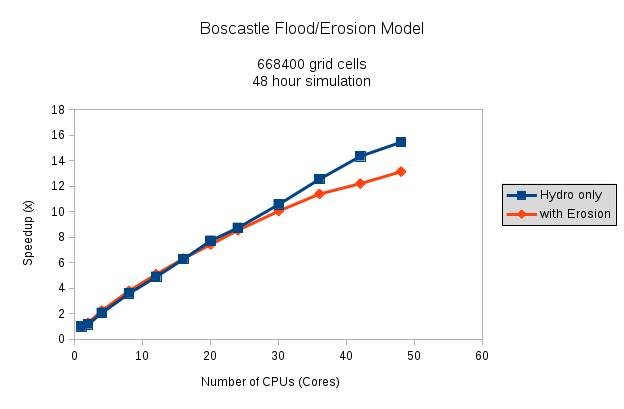
As a lot of the code has sections that have to be done serially, there’s not a 1:1 scaling of CPUs to speed-up-multiplier, which is to be expected. But I’m quite happy with this for now; if I’ve got time at some point, I’ll delve into OpenMP some more and look for other areas of the code to parallelise. Obviously the simulations with the erosion routines switched on take a lot longer to do: They don’t parallelise quite so well, and there’s a lot more computation with all the different grain sizes etc. While the hydro model speed up is roughly linear all the way up to around 48 cores (you can just see it tailing off perhaps around 40 cores…) the erosion simulations speed-up clearly starts to tail off around 24 cores upwards.

The actual run times can be compared with the graph below:

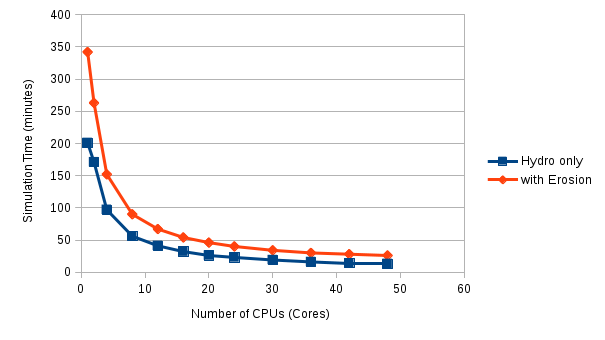
Actual run times with erosion routines on are approaching double that with just the hydrological model, in serial. However as both codes scale up over more CPUs, the gap narrows, relatively speaking. All these simulations are run with around 600000 grid cells (a 5m resolution DEM). Future work will look at some larger model domains to see how this affects scaling. (Spoiler alert: guess what, it does!)