1. Quickstart
We have developed a toolkit to automate calculation of basin (or catchement) averaged denudation rates estimated from the concentration of in situ cosmogenic nuclides in stream sediment. This toolkit is called the CAIRN method. Currently 10Be and 26Al are supported.
If you use this to calculate denudation rates that are later published, please cite this paper:
Mudd, S. M., Harel, M.-A., Hurst, M. D., Grieve, S. W. D., and Marrero, S. M.: The CAIRN method: automated, reproducible calculation of catchment-averaged denudation rates from cosmogenic nuclide concentrations, Earth Surf. Dynam., 4, 655-674, doi:10.5194/esurf-4-655-2016, 2016.
The toolkit requires:
-
Data on cosmogenic samples.
-
A file containing filenames of the topographic data, and optional filenames for shielding rasters.
-
A parameter file.
The toolkit then produces:
-
A csv file that contains results of the analysis.
-
A text file that can be copied into the CRONUS online calculator for data comparison.
2. Introduction
This takes you through the process of calculating erosion rates from 10Be or 26Al
3. Get the code and data basin-averaged cosmogenic analysis
This section goes walks you through getting the code and example data, and also describes the different files you will need for the analysis.
3.1. Get the source code for basin-averaged cosmogenics
First navigate to the folder where you will keep your repositories.
In this example, that folder is called /home/LSDTT_repositories.
In a terminal window, go there with the cd command:
$ cd /home/LSDTT_repositories/You can use the pwd command to make sure you are in the correct directory.
If you don’t have the directory, use mkdir to make it.
3.1.1. Clone the code from Git
Now, clone the repository from GitHub:
$ pwd
/home/LSDTT_repositories/
$ git clone https://github.com/LSDtopotools/LSDTopoTools_CRNBasinwide.git
Alternatively, get the zipped code
If you don’t want to use git, you can download a zipped version of the code:
$ pwd
/home/LSDTT_repositories/
$ wget https://github.com/LSDtopotools/LSDTopoTools_CRNBasinwide/archive/master.zip
$ gunzip master.zip
GitHub zips all repositories into a file called master.zip,
so if you previously downloaded a zipper repository this will overwrite it.
|
3.1.2. Compile the code
Okay, now you should have the code. You will still be sitting in the directory
/home/LSDTT_repositories/, so navigate up to the directory LSDTopoTools_BasinwideCRN/driver_functions_BasinwideCRN/.
$ pwd
/home/LSDTT_repositories/
$ cd LSDTopoTools_CRNBasinwide
$ cd driver_functions_CRNBasinwide
There are a number of makefiles (thse with extension .make in this folder).
These do a number of different things that will be explained later in this chapter.
3.2. Getting example data: The San Bernardino Mountains
We have provided some example data. This is on our Github example data website.
The example data has a number of digital elevation models in various formats, but for these examples we will be only using one dataset, from the San Bernardino Mountains in California.
You should make a folder for your data using mkdir somewhere sensible.
For the purposes of this tutorial I’ll put it in the following folder:
$ pwd
/home/ExampleDatasets/SanBernardino/
Again, we will only take the data we need, so use wget to download the data:
$ wget https://github.com/LSDtopotools/ExampleTopoDatasets/raw/master/SanBern.bil
$ wget https://github.com/LSDtopotools/ExampleTopoDatasets/raw/master/SanBern.hdr
$ wget https://github.com/LSDtopotools/ExampleTopoDatasets/raw/master/example_parameter_files/SanBern_CRNData.csv
$ wget https://github.com/LSDtopotools/ExampleTopoDatasets/raw/master/example_parameter_files/SanBern_CRNRasters.csv
$ wget https://github.com/LSDtopotools/ExampleTopoDatasets/raw/master/example_parameter_files/SanBern.CRNParam
You should now have the following files in your data folder:
$ pwd
/home/ExampleDatasets/SanBernardino/
$ ls
SanBern.bil    SanBern_CRNData.csv     SanBern.CRNParam
SanBern.hdr    SanBern_CRNRasters.csv
The file SanBern_CRNRasters.csv will need to be modified with the appropriate paths to your files! We will describe how to do that below.
|
3.3. Setting up your data directories and parameter files
Before you can run the code, you need to set up some data structures.
| If you downloaded the example data, these files will already exist. These instructions are for when you need to run CRN analysis on your own datasets. |
-
You can keep your topographic data separate from your cosmogenic data, if you so desire. You’ll need to know the directory paths to these data.
-
In a single folder (again, it can be separate from topographic data), you must put a i) parameter file, a cosmogenic data file, and a raster filenames file .
-
These three files must have the same prefix, and each have their own extensions.
-
The parameter file has the extension:
.CRNParam. -
The cosmogenic data file has the extension
_CRNData.csv. -
The raster filenames file has the extension
_CRNRasters.csv.
-
-
For example, if the prefix of your files is
SanBern, then your three data files will beSanBern.CRNParam,SanBern_CRNData.csv, andSanBern_CRNRasters.csv. -
If the files do not have these naming conventions, the code WILL NOT WORK! Make sure you have named your files properly.
3.3.1. The parameter file
The parameter file contains some values that are used in the calculation of both shielding and erosion rates.
This file must have the extension .CRNParam. The extension is case sensitive.
|
The parameter file could be empty, in which case parameters will just take default values. However, you may set various parameters. The format of the file is:
parameter_name: parameter_valueSo for example a parameter file might look like:
min_slope: 0.0001
source_threshold: 12
search_radius_nodes: 1
threshold_stream_order: 1
theta_step: 30
phi_step: 30
Muon_scaling: Braucher
write_toposhield_raster: true
write_basin_index_raster: true
There cannot be a space between the parameter name and the ":" character,
so min_slope : 0.0002 will fail and you will get the default value.
|
In fact all of the available parameters are listed above, and those listed above are default values. The parameter names are not case sensitive. The parameter values are case sensitive. These parameters are as follows:
| Keyword | Input type | default | Description |
|---|---|---|---|
min_slope |
float |
0.0001 |
The minimum slope between pixels used in the filling function (dimensionless) |
source_threshold |
int |
12 |
The number of pixels that must drain into a pixel to form a channel. This parameter makes little difference, as the channel network only plays a role in setting channel pixels to which cosmo samples will snap. This merely needs to be set to a low enough value that ensures there are channels associated with each cosmogenic sample. |
search_radius_nodes |
int |
1 |
The number of pixels around the location of the cosmo location to search for a channel. The appropriate setting will depend on the difference between the accuracy of the GPS used to collect sample locations and the resolution of the DEM. If you are using a 30 or 90m DEM, 1 pixel should be sufficient. More should be used for LiDAR data. |
threshold_stream_order |
int |
1 |
The minimum stream or which the sample snapping routine considers a 'true' channel. The input is a Strahler stream order. |
theta_step |
int |
30 |
Using in toposhielding calculations. This is the step of azimuth (in degrees) over which shielding and shadowing calculations are performed. Codilean (2005) recommends 5, but it seems to work without big changes differences with 15. An integer that must be divisible by 360 (although if not the code will force it to the closest appropriate integer). |
phi_step |
int |
30 |
Using in toposhielding calculations. This is the step of inclination (in degrees) over which shielding and shadowing calculations are performed. Codilean (2005) recommends 5, but it seems to work without big changes differences with 10. An integer that must be divisible by 360 (although if not the code will force it to the closest appropriate integer). |
path_to_atmospheric_data |
string |
./ |
The path to the atmospheric data. DO NOT CHANGE. This is included in the repository so should work if you have cloned our git repository. Moving this data and playing with the location the atmospheric data is likeley to break the program. |
Muon_scaling |
string |
Braucher |
The scaling scheme for muons. Options are "Braucher", "Schaller" and "Granger". If you give the parameter file something other than this it will default to Braucher scaling. These scalings take values reported in COSMOCALC as described by Vermeesch 2007. |
write_toposhield_raster |
bool |
true |
If true this writes a toposhielding raster if one does not exist. Saves a bit of time but will take up some space on your hard disk! |
write_basin_index_raster |
bool |
true |
For each DEM this writes an LSDIndexRaster to file with the extension |
write_full_scaling_rasters |
bool |
true |
This writes three rasters if true: a raster with |
3.3.2. The cosmogenic data file
This file contains the actual cosmogenic data: it has the locations of samples, their concentrations of cosmogenics (10Be and 26Al) and the uncertainty of these concentrations.
The cosmogenic data file must have the extension _CRNData.csv.
The extension is case sensitive.
|
This is a .csv file: that is a comma separated value file. It is in that format to be both excel and
pandas friendly.
The first row is a header that names the columns, after that there should be 7 columns (separated by commas) and unlimited rows. The seven columns are:
sample_name, sample_latitude, sample_longitude, nuclide, concentration, AMS_uncertainty, standardisation
An example file would look like this (this is not real data):
Sample_name,Latitude,Longitude,Nuclide,Concentration,Uncertainty,Standardisation
LC07_01,-32.986389,-71.4225,Be10,100000,2500,07KNSTD
LC07_04,-32.983528,-71.415556,Be10,150000,2300,07KNSTD
LC07_06,-32.983028,-71.415833,Al26,4000,2100,KNSTD
LC07_08,-32.941333,-71.426583,Be10,30000,1500,07KNSTD
LC07_10,-33.010139,-71.435389,Be10,140000,25000,07KNSTD
LC07_11,-31.122417,-71.576194,Be10,120502,2500,07KNSTD
Or, with reported snow shielding:
Sample_name,Latitude,Longitude,Nuclide,Concentration,Uncertainty,Standardisation, Snow_shielding
LC07_01,-32.986389,-71.4225,Be10,100000,2500,07KNSTD,0.7
LC07_04,-32.983528,-71.415556,Be10,150000,2300,07KNSTD,0.8
LC07_06,-32.983028,-71.415833,Al26,4000,2100,KNSTD,1.0
LC07_08,-32.941333,-71.426583,Be10,30000,1500,07KNSTD,1.0
LC07_10,-33.010139,-71.435389,Be10,140000,25000,07KNSTD,1.0
LC07_11,-31.122417,-71.576194,Be10,120502,2500,07KNSTD,0.987
If you followed the instructions earlier in the section Getting example data: The San Bernardino Mountains
then you will have a CRNdata.csv file called Binnie_CRNData.csv in your data folder.
| Column | Heading | type | Description |
|---|---|---|---|
1 |
Sample_name |
string |
The sample name NO spaces or underscore characters! |
2 |
Latitude |
float |
Latitude in decimal degrees. |
3 |
Longitude |
float |
Longitude in decimal degrees. |
4 |
Nuclide |
string |
The nuclide. Options are |
5 |
Concentration |
float |
Concentration of the nuclide in atoms g-1. |
6 |
Uncertainty |
float |
Uncertainty of the concentration of the nuclide in atoms g-1. |
7 |
Standardization |
float |
The standardization for the AMS measurments. See table below for options. |
8 |
Reported snow shielding |
float |
The reported snow shielding value for a basin. Should be a ratio between 0 (fully shielded) and 1 (no shielding). This column is OPTIONAL. |
| Nuclide | Options |
|---|---|
10Be |
|
26Al |
|
3.3.3. The raster names file
This file contains names of rasters that you want to analyze.
The raster names file must have the extension _CRNRasters.csv.
The extension is case sensitive.
|
This file is a csv file that has as many rows as you have rasters that cover your CRN data. Each row can contain between 1 and 4 columns.
-
The first column is the FULL path name to the Elevation raster and its prefix (that is, without the
.bil, e.g.:/home/smudd/basin_data/Chile/CRN_basins/Site01/Site_lat26p0_UTM19_DEM -
The next column is either a full path name to a snow shielding raster or a snow shielding effective depth. Both the raster and the single value should have units of g/cm^2 snow depth. If there is no number here the default is 0.
-
The next column is either a full path name to a self shielding raster or a self shielding effective depth. Both the raster and the single value should have units of g/cm2 shielding depth. If there is no number here the default is 0.
-
The next column is the FULL path to a toposhielding raster. If this is blank the code will run topographic shielding for you.
topographic shielding is the most computationally demanding step in the cosmo analysis. A typical file might will look like this:
An example CRNRasters.csv file/home//basin_data/Site01/Site01_DEM,0,0,/home/basin_data/Site01/Site01_DEM_TopoShield /home/basin_data/Site02/Site02_DEM,5,10 /home/basin_data/Site03/Site03_DEM,5,/home/basin_data/Site03/Site03_DEM_SelfShield /home/basin_data/Site04/Site04_DEM,/home/basin_data/Site04/Site04_DEM_SnowShield,/home/basin_data/Site04/Site04_DEM_SelfShield /home/basin_data/Site05/Site05_DEM /home/basin_data/Site06/Site06_DEM,/home/basin_data/Site06/Site06_DEM_SnowShield
| Column | Heading | type | Description |
|---|---|---|---|
1 |
Path and prefix of elevation data |
string |
Path and prefix of elevation data; does not include the extension (that is, does not include |
2 |
Snow shielding |
float or string or empty |
This could be empty, or contain a float, in which case it is the effective depth of snow (g cm-2) across the entire basin or a string with the path and file prefix of the snow depth (g cm-2) raster. If empty, snow depth is assumed to be 0. |
3 |
Self shielding |
float or string or empty |
This could be empty, or contain a float, in which case it is the effective depth of material eroded(g cm-2) across the entire basin or a string with the path and file prefix of the eroded depth (g cm-2) raster. If empty, eroded depth is assumed to be 0. |
4 |
Topo shielding |
string or empty |
This could be empty or could contain a string with the path and file prefix of the topographic shielding (a ratio between 0 and 1) raster. If empty topographic shielding is assumed to be 1 (i.e., no shielding). |
3.4. Modifying your CRNRasters file the python way
The _CRNRasters.csv file contains the path names and the file prefixes of the rasters to be used in the analysis.
The paths will vary depending on your own file structures.
Updating these paths by hand can be quite tedious, so we have prepared a python script to automate this process.
You can get this script here:
$ wget https://github.com/LSDtopotools/LSDAutomation/raw/master/LSDOSystemTools.py
$ wget https://github.com/LSDtopotools/LSDAutomation/raw/master/PrepareCRNRastersFileFromDirectory.pyThe script LSDOSystemTools.py contians some tools for managing paths and files, the actual work is done by the script PrepareCRNRastersFileFromDirectory.py.
In an editor, go into PrepareCRNRastersFileFromDirectory.py and navigate to the bottom of the file.
Change the path to point to the directory with your DEMs. The prefix is the prefix of your files, so in this example change prefix to SanBern.
You can then run the script with:
$ python PrepareCRNRastersFileFromDirectory.pyThis script will then update the _CRNRasters.csv file to reflect your directory structure. The script also detects any associated shielding rasters.
4. Calculating Topographic Shielding
Cosmogenic nuclides are produced at or near the Earth’s surface by cosmic rays, and these rays can be blocked by topography (i.e., big mountains cast "shadows" for cosmic rays).
In most cases, you will not have topographic shielding rasters available, and will need to calculate these.
Shielding calculation are computationally intensive, much more so than the actual erosion rate computations. Because of the computational expense of shielding calculations, we have prepared a series of tools for speeding this computation.
The topographic shielding routines take the rasters from the _CRNRasters.csv file and the _CRNData.csv file and computes the location of all CRN basins.
They then clips a DEM around the basins (with a pixel buffer set by the user).
These clipped basins are then used to make the shielding calculations and the erosion rate calculations.
This process of clipping out each basin spans a large number of new DEM that require a new directory structure. A python script is provided to set up this directory structure in order to organize the new rasters.
| This process uses a large amount of storage on the hard disk because a new DEM will be written for each CRN basin. |
4.1. Steps for preparing the rasters for shielding calculations
4.1.1. Creation of subfolders for your topographic datasets
The first step is to create some subfolders to store topographic data. We do this using a python script
-
First, place the
_CRNRasters.csvand_CRNData.csvfile into the same folder, and make sure the_CRNRasters.csvfile points to the directories that contain the topographic data. If you are working with the example data (see section Getting example data: The San Bernardino Mountains), you should navigate to the folder with the data (for this example, the folder is in/home/ExampleDatasets/SanBernardino/):$ pwd /home/ExampleDatasets/SanBernardino/ $ ls SanBern_CRNData.csv SanBern_CRNRasters.csv SanBern.hdr SanBern.bil SanBern.CRNparamYou will then need to modify
SanBern_CRNRasters.csvto reflect your directory:Modify yourSanBern_CRNRasters.csvfile/home/ExampleDatasets/SanBernardino/SanBernEach line in this file points to a directory holding the rasters to be analyzed.
In this case we are not supplying and shielding rasters. For more details about the format of this file see the section: The raster names file.
-
Second, run the python script
PrepareDirectoriesForBasinSpawn.py.-
You can clone this script from GitHub; find it here: https://github.com/LSDtopotools/LSDAutomation You will also need the file
LSDOSystemTools.pyfrom this repository. TheLSDOSystemTools.pyfile contains some scripts for making sure directories are in the correct format, and for changing filenames if you happen to be switching between Linux and Windows. It is unlikely that you will need to concern yourself with its contents, as long as it is present in the same folder as thePrepareDirectoriesForBasinSpawn.pyfile.The scripts can be downloaded directly using:
$ wget https://github.com/LSDtopotools/LSDAutomation/raw/master/PrepareDirectoriesForBasinSpawn.py $ wget https://github.com/LSDtopotools/LSDAutomation/raw/master/LSDOSystemTools.py -
You will need to scroll to the bottom of the script and change the
path(which is simply the directory path of the_CRNRasters.csvfile. -
You will need to scroll to the bottom of the script and change the
prefix(which is simply prefix of the_CRNRasters.csvfile; that is the filename before_CRNRasters.csvso if the filename isYoYoMa_CRNRasters.csvthenprefixisYoYoMa. Note this is case sensitive.In this example, scroll to the bottom of the file and change it to:
if __name__ == "__main__": path = "/home/ExampleDatasets/SanBernardino" prefix = "SanBern" PrepareDirectoriesForBasinSpawn(path,prefix) -
This python script does several subtle things like checking directory paths and then makes a new folder for each DEM. The folders will contain all the CRN basins located on the source DEM.
If you are using the example data, the rather trivial result will be a directory called
SanBern.
-
4.1.2. Spawning the basins
Now you will run a C++ program that spawns small rasters that will be used for shielding calculations. First you have to compile this program.
-
To compile, navigate to the folder
/home/LSDTT_repositories/LSDTopoTools_CRNBasinwide/driver_functions_CRNBasinwide/. If you put the code somewhere else, navigate to that folder. Once you are in the folder with the driver functions, type:$ make -f Spawn_DEMs_for_CRN.make -
The program will then compile (you may get some warnings—ignore them.)
-
In the
/driver_functions_CRNTools/folder, you will now have a programSpawn_DEMs_for_CRN.exe. You need to give this program two arguments. -
You need to give
Spawn_DEMs_for_CRN.exe, the path to the data files (i.e.,_CRNRasters.csvand_CRNData.csv), and the prefix, so if they are calledYoMa_CRNRaster.csvthe prefix isYoMa). In this example the prefix will beSanBern. Run this with:PS> Spawn_DEMs_for_CRN.exe PATHNAME DATAPREFIXin windows or:
$ ./Spawn_DEMs_for_CRN.exe PATHNAME DATAPREFIXin Linux.
In our example, you should run:
$ ./Spawn_DEMs_for_CRN.exe /home/ExampleDatasets/SanBernardino/ SanBernThe PATHNAME MUST have a frontslash at the end. /home/ExampleDatasets/SanBernardino/will work whereas/home/ExampleDatasets/SanBernardinowill lead to an error. -
Once this program has run, you should have subfolders containing small DEMs that contain the basins to be analyzed. There will be one for every cosmogenic sample that lies within the DEM.
-
You will also have files that contain the same
PATHNAMEandPREFIXbut have_Spawnedadded to the prefix. For example, if your original prefix wasCRN_test, the new prefix will beCRN_test_Spawned. -
In the file
PREFIX_Spawned_CRNRasters.csvyou will find the paths and prefixes of all the spawned basins.
4.2. The shielding computation
The shielding computation is the most computationally expensive step of the CRN data analysis. Once you have spawned the basins (see above section, Steps for preparing the rasters for shielding calculations), you will need to run the shielding calculations.
-
You will first need to compile the program that calculates shielding. This can be compiled with:
$ make -f Shielding_for_CRN.make -
The compiled program (
Shielding_for_CRN.exe) takes two arguments: thePATHNAMEand thePREFIX. -
You could simply run this on a single CPU after spawning the basins; for example if the original data had the prefix
CRN_testbefore spawning, you could run the program with:$ ./Shielding_for_CRN.exe PATHNAME CRN_test_Spawnedwhere
PATHNAMEis the path to your_CRNRasters.csv,_CRNData.csv, and.CRNParam(these files need to be in the same path).If you only wanted to do a subset of the basins, you can just delete rows from the *_Spawned_CRNRasters.csvfile as needed.
This will produce a large number of topographic shielding rasters (with _SH in the filename), for example:
smudd@burn SanBern $ ls
SpawnedBasin_10.bil SpawnedBasin_17.bil SpawnedBasin_7.bil SpawnedBasin_MHC-13.bil
SpawnedBasin_10.hdr SpawnedBasin_17.hdr SpawnedBasin_7.hdr SpawnedBasin_MHC-13.hdr
SpawnedBasin_11.bil SpawnedBasin_18.bil SpawnedBasin_8.bil SpawnedBasin_MHC-14.bil
SpawnedBasin_11.hdr SpawnedBasin_18.hdr SpawnedBasin_8.hdr SpawnedBasin_MHC-14.hdr
SpawnedBasin_12.bil SpawnedBasin_19.bil SpawnedBasin_9.bil SpawnedBasin_MHC-15.bil
SpawnedBasin_12.hdr SpawnedBasin_19.hdr SpawnedBasin_9.hdr SpawnedBasin_MHC-15.hdr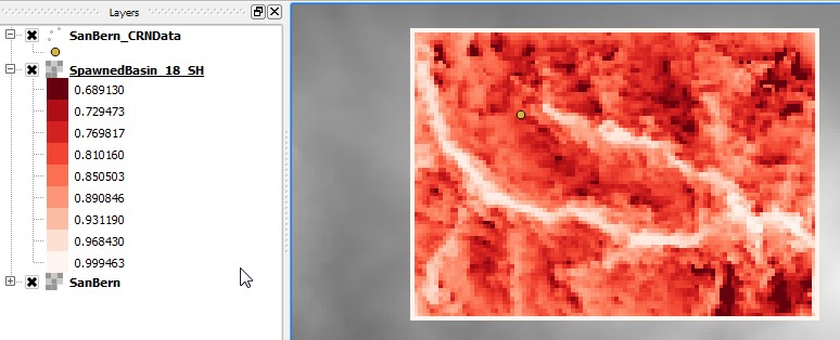
18) from the San Bernardino dataset (viewed in QGIS2.2)4.3. Embarrassingly parallel shielding
We provide a python script for running multiple basins using an embarrassingly parallel approach.
It is written for our cluster:
if your cluster uses qsub or equivalent, you will need to write your own script.
However, this will work on systems where you can send jobs directly.
-
To set the system up for embarrassingly parallel runs, you need to run the python script
ManageShieldingComputation.py, which can be found here: https://github.com/LSDtopotools/LSDAutomation. You can download it with:$ wget https://github.com/LSDtopotools/LSDAutomation/raw/master/ManageShieldingComputation.py -
In
ManageShieldingComputation.py, navigate to the bottom of the script, and enter thepath,prefix, andNJobs.NJobsis the number of jobs into which you want to break up the shielding computation. -
Once you run this computation, you will get files with the extension
_bkNNwhereNNis a job number. -
In addition a text file is generated, with the extension
_ShieldCommandPrompt.txt, and from this you can copy and paste job commands into a Linux terminal.These commands are designed for the GeoSciences cluster at the University of Edinburgh: if you use qsubyou will need to write your own script. -
Note that the parameters for the shielding calculation are in the
.CRNParamfiles. We recommend:theta_step:8 phi_step: 5These are based on extensive sensitivity analyses and balance computational speed with accuracy. Errors will be << 1% even in landscapes with extremely high relief. Our forthcoming paper has details on this.
-
Again, these computations take a long time. Don’t start them a few days before your conference presentation!!
-
Once the computations are finished, there will be a shielding raster for every spawned basin raster. In addition, the
_CRNRasters.csvfile will be updated to reflect the new shielding rasters so that the updated parameter files can be fed directly into the erosion rate calculators.
4.4. Once you have finished with spawning and topographic shielding calculations
If you are not going to assimilate reported snow shielding values, you can move on to the erosion rate calculations. If you are going to assimilate reported snow shielding values, please read the section: Using previously reported snow shielding.
4.5. Stand alone topographic shielding calculations
We also provide a stand alone program just to calculate topographic shielding. This may be useful for samples collected for measuring exposure ages or for working in other settings such as active coastlines.
-
You will first need to compile the program that calculates topographic shielding. This can be compiled with:
$ make -f TopoShielding.make -
The compiled program (
TopoShielding.out) takes four arguments: thePATHNAME, thePREFIX, theAZIMUTH STEPand theANGLE STEP. -
You could simply run this on a single CPU; for example if the original DEM had the prefix
CRN_TESTbefore spawning, and you wanted to use anAZIMUTH_STEP=5andANGLE_STEP=5, you could run the program with:$ ./TopoShielding.out PATHNAME CRN_TEST 5 5where
PATHNAMEis the path to yourCRN_TEST.The DEM must be in ENVI *.bil format. See information about LSDTopoTools data formats.
This will produce a single topographic shielding raster (with _TopoShield in the filename).
5. Snow shielding calculations
Snow absorbs cosmic rays and so CRN concentrations in sediments can be affected by snow that has been present in the basin during the period that eroded materials were exposed to cosmic rays.
Estimating snow shielding is notoriously difficult (how is one to rigorously determine the thickness of snow averaged over the last few thousand years?), and our software does not prescribe a method for calculating snow shielding.
Rather, our tools allow the user to set snow shielding in 3 ways:
-
Use a previously reported basinwide average snow shielding factor
-
Assign a single effective average depth of snow over a catchment (in g cm-2).
-
Pass a raster of effective average depth of snow over a catchment (in g cm-2).
5.1. Using previously reported snow shielding
Some authors report a snow shielding factor in their publications. The underlying information about snow and ice thickness used to generate the snow shielding factor is usually missing. Because under typical circumstances the spatial distribution of snow thicknesses is not reported, we use reported snow shielding factors to calculate an effective snow thickness across the basin.
This approach is only compatible with our spawning method (see the section on Spawning the basins), because this average snow thickness will only apply to the raster containing an individual sample’s basin.
The effective snow thickness is calculated by:
where \(d_{eff}\) is the effective depth (g cm-2), \(\Gamma_0\) is the attenuation mass (= 160 g cm-2) for spallation (we do not consider the blocking of muons by snow), and, \(S_s\) is the reported snow shielding.
The reported snow shielding values should be inserted as the 8th column in the CRNData.csv file.
For example,
Sample_name,Latitude,Longitude,Nuclide,Concentration,Uncertainty,Standardisation,Snow_shield
20,34.3758,-117.09,Be10,215100,9400,07KNSTD,0.661531836
15,34.3967,-117.076,Be10,110600,7200,07KNSTD,0.027374149
19,34.4027,-117.063,Be10,84200,6500,07KNSTD,0.592583113
17,34.2842,-117.056,Be10,127700,5800,07KNSTD,0.158279369
14,34.394,-117.054,Be10,101100,6100,07KNSTD,0.047741051
18,34.2794,-117.044,Be10,180600,10000,07KNSTD,0.559339639
11,34.1703,-117.044,Be10,7700,1300,07KNSTD,0.210018127
16,34.2768,-117.032,Be10,97300,5500,07KNSTD,0.317260607
10,34.2121,-117.015,Be10,74400,5200,07KNSTD,0.2538638435.1.1. Steps to use reported snow shielding
Reported snow shielding values are done on a basin-by-basin basis, so our snow shielding must have individual shielding calculations for each sample. This is only possible using our "spawning" routines.
-
The spawning of basins must be performed: see Spawning the basins
-
The
*_spawned_CRNData.csvshould have snow shielding values in the 8th column. -
A python script,
JoinSnowShielding.py, must be run that translates reported snow shielding values into effective depths. This script, and a required helper script,LSDOSystemTools.pycan be downloaded from:$ wget https://github.com/LSDtopotools/LSDAutomation/raw/master/JoinSnowShielding.py $ wget https://github.com/LSDtopotools/LSDAutomation/raw/master/LSDOSystemTools.pyYou will need to scroll to the bottom of the
JoinSnowShielding.pyprogram and edit both the path name and the file prefix. For example, if your spawned data was in/home/ExampleDatasets/SanBernardino/and the files wereSanBern_spawned_CRNRasters.csv,SanBern_spawned_CRNData.csv, andSanBern_spawned.CRNParam, then the bottom of the python file should contain:if __name__ == "__main__": path = "/home/ExampleDatasets/SanBernardino" prefix = "SanBern_spawned" GetSnowShieldingFromRaster(path,prefix) -
This script will then modify the
*spawned_CRNRasters.csvso that the second column will have an effective snow shiedling reflecting the reported snow shielding value (converted using the equation earlier in this section). It will print a new file,*spawned_SS_CRNRasters.csvand copy the CRNData and CRNParam files to ones with prefixes:*_spawned_SS_CRNData.csvand*_spawned_SS.CRNParam. -
These new files (with
_SSin the prefix) will then be used by the erosion rate calculator.
5.2. Assign a single effective average depth
This option assumes that there is a uniform layer of time-averaged snow thickness over the entire basin. The thickness reported is in effective depth (g cm-2).
To assign a constant thickness, one simply must set the section column of *_CRNRasters.csv file to the appropriate effective depth.
For example, a file might look like:
/home/topodata/SanBern,15
/home/topodata/Sierra,15,0
/home/topodata/Ganga,15,0,/home/topodata/Ganga_shieldedIn the above example the first row just sets a constant effective depth of 15 g cm-2, The second also assigns a self shielding value of 0 g cm-2 (which happens to be the default), and the third row additionally identifies a topographic shielding raster.
In general, assigning a constant snow thickness over the entire DEM is not particularly realistic, and it is mainly used to approximate the snow shielding reported by other authors when they have not made the spatially distributed data about snow thicknesses available see Using previously reported snow shielding.
5.3. Pass a raster of effective average depth of snow over a catchment
Our software also allows users to pass a raster of effective snow thicknesses (g cm-2). This is the time-averaged effective thickness of snow which can be spatially heterogeneous.
The raster is given in the second column of the *_CRNRasters.csv, so, for example in the below file the 4th and 6th rows point to snow shielding rasters.
/home//basin_data/Site01/Site01_DEM,0,0,/home/basin_data/Site01/Site01_DEM_TopoShield
/home/basin_data/Site02/Site02_DEM,5,10
/home/basin_data/Site03/Site03_DEM,5,/home/basin_data/Site03/Site03_DEM_SelfShield
/home/basin_data/Site04/Site04_DEM,/home/basin_data/Site04/Site04_DEM_SnowShield,/home/basin_data/Site04/Site04_DEM_SelfShield
/home/basin_data/Site05/Site05_DEM
/home/basin_data/Site06/Site06_DEM,/home/basin_data/Site06/Site06_DEM_SnowShield| The snow shielding raster must be the same size and shape as the underlying DEM (i.e. they must have the same number of rows and columns, same coordinate system and same data resolution). |
| These rasters need to be assigned BEFORE spawning since the spawning process will clip the snow rasters to be the same size as the clipped topography for each basin. |
5.4. Compute snow shielding from snow water equivalent data
In some cases you might have to generate the snow shielding raster yourself. We have prepared some python scripts and some C++ programs that allow you to do this.
-
First, you need to gather some data. You can get the data from snow observations, or from reconstructions. The simple functions we have prepared simply approximate snow water equivalent (SWE) as a function of elevation.
-
You need to take your study area, and prepare a file that has two columns, seperated by a space. The first column is the elevation in metres, and the second column is the average annual snow water equivalent in mm. Here is an example from Idaho:
968.96 70.58333333 1211.2 16 1480.692 51.25 1683.568 165.8333333 1695.68 115.4166667 1710.82 154.1666667 1877.36 139.75 1925.808 195.1666667 1974.256 277.75 2240.72 253.0833333 2404.232 241.5833333 2395.148 163.0833333 -
Once you have this file, download the following python script from our repository:
$ wget https://github.com/LSDtopotools/LSDTopoTools_CRNBasinwide/raw/master/SnowShieldFit.py -
Open the python file and change the filenames to reflect the name of your data file withing the python script, here (scroll to the bottom):
if __name__ == "__main__":

    # Change these names to create the parameter file.  The first line is the name
    # of the data file and the second is the name of the parameter file
    filename = 'T:\\analysis_for_papers\\Manny_idaho\\SWE_idaho.txt'
    sparamname = 'T:\\analysis_for_papers\\Manny_idaho\\HarringCreek.sparam'
This script will fit the data to a bilinear function, shown to approximate the SWE distribution with elevation in a number of sites. You can read about the bilinear fit in a paper by Kirchner et al., HESS, 2014 and by Grünewald et al., Cryosphere, 2014.
For reasons we will see below the prefix (that is the pit before the
.sparam) should be the same as the name of the elevation DEM upon which the SWE data will be based. -
Run the script with:
$ python SnowShieldFit.py -
This will produce a file with the extension sparam. The .sparam file contains the slope and intercept for the annual average SWE for the two linear segments, but in units of g cm-2. These units are to ensure the snow water equivalent raster is in units compatible with effective depths for cosmogenic shielding.
The data file you feed in to SnowShieldFit.pyshould have SWE in mm, whereas the snow shielding raster will have SWE in effective depths with units g cm-2. -
Okay, we can now use some C++ code to generate the snow shielding raster. If you cloned the repository (using
git clone https://github.com/LSDtopotools/LSDTopoTools_AnalysisDriver.git), you will have a function for creating a snow shielding raster. Navigate to thedriver_functionsfolder and make the program using:$ make -f SimpleSnowShield.make -
You run this program with two arguments. The first argument is the path to the
.sparamfile that was generated by the scriptSnowShieldFit.py. The path MUST include a final slash (i.e./home/a/directory/will work but/home/a/directorywill fail.) The second argument is the prefix of the elevation DEM AND the.sparamfile (i.e. if the file isHarringCreek.sparamthen the prefix isHarringCreek). The code will then print out anbilformat raster with the prefix plus_SnowBLso for example if the prefix isHarringCreekthen the output raster isHarringCreek_SnowBL.bil. The command line would look something like:$ ./The prefix of the .sparamfile MUST be the same as the DEM prefix. -
Congratulations! You should now have a snow shielding raster that you can use in your CRN-based denudation rate calculations. NOTE: The program
SimpleSnowShield.execan also produce SWE rasters using a modified Richard’s equation, which has been proposed by Tennent et al., GRL, but at the moment we do not have functions that fit SWE data to a Richard’s equation so this is only recommended for users with pre-calculated parameters for such equations. -
If you have performed this step after spawning the DEMs (see the section Spawning the basins), you can update the
_CRNRasters.csvby running the python scriptPrepareCRNRastersFileFromDirectory.py, which you can read about in the section: Modifying your CRNRasters file the python way.
6. Calculating denudation rates
Okay, now you are ready to get the denudation rates.
You’ll need to run the function from the directory where the compiled code is located
(in our example, /home/LSDTT_repositories/LSDTopoTools_CRNBasinwide/), but it can work on data in some arbitrary location.
6.1. Compiling the code
To compile the code, go to the driver function folder
(in the example, /home/LSDTT_repositories/LSDTopoTools_CRNBasinwide/driver_functions_CRNBasinwide)
and type:
$ make -f Basinwide_CRN.makeThis will result in a program called Basinwide_CRN.exe.
6.2. Running the basin averaged denudation rate calculator
$ ./Basinwide_CRN.exe pathname_of_data file_prefix method_flag-
The pathname_of_data is just the path to where your data is stored, in this example that is
/home/ExampleDatasets/SanBernardino/.You MUST remember to put a /at the end of your pathname. -
The filename is the PREFIX of the files you need for the analysis (that is, without the extension).
-
In the example this prefix is
SanBern. -
If you want to use the spawned basins used
SanBern_Spawned. -
If you spawned basins and calculated shielding the prefix is
SanBern_spawned_Shield
-
-
The
method_flagtells the program what method you want to use to calculate erosion rates. The options are:
| Flag | Description |
|---|---|
0 |
A basic analysis that does not include any shielding (i.e., no topographic, snow or self shielding). |
1 |
An analysis that includes shielding, but does not account for spawning (see Spawning the basins for details on spawning). If this option is used on spawned basins it is likely to result in errors. Note that spawning speeds up calculations if you have multiple processors at your disposal, but |
2 |
An analyis that includes shielding, to be used on spawned basins (see Spawning the basins for details on spawning). This is the default. |
6.3. The output files
There are two output files. Both of these files will end up in the pathname that you designated when calling the program.
The first is called file_prefix_CRNResults.csv and the second is called file_prefix_CRONUSInput.txt
where file_prefix is the prefix you gave when you called the program.
So, for example, if you called the program with:
$ ./basinwide_CRN.exe /home/ExampleDatasets/SanBernardino/ SanBernThe outfiles will be called:
SanBern_CRNResults.csv
SanBern_CRONUSInput.txt
The _CRONUSInput.txt is formatted to be cut and pasted directly into the CRONUS calculator.
The file has some notes (which are pasted into the top of the file):
->IMPORTANT nuclide concentrations are not original!
      They are scaled to the 07KNSTD!!
->Scaling is averaged over the basin for snow, self and topographic shielding.
->Snow and self shielding are considered by neutron spallation only.
->Pressure is an effective pressure that reproduces Stone scaled production
      that is calculated on a pixel by pixel basis.
->Self shielding is embedded in the shielding calculation and so
sample thickness is set to 0.| You should only paste the contents of the file below the header into the CRONUS calculator, which can be found here: http://hess.ess.washington.edu/math/al_be_v22/al_be_erosion_multiple_v22.php A new version of the CRONUS caluclator should be available late 2016 but should be backward compatible with the prior version. See here: http://hess.ess.washington.edu/math/index_dev.html |
The _CRNResults.csv is rather long.
It contains the following data in comma separated columns:
| Column | Name | Units | Description |
|---|---|---|---|
1 |
basinID |
Integer |
A unique identifier for each CRN sample. |
2 |
sample_name |
string |
The name of the sample |
3 |
Nuclide |
string |
The name of the nuclide. Must be either |
4 |
latitude |
decimal degrees |
The latitude. |
5 |
longitude |
decimal degrees |
The longitude. |
6 |
concentration |
atoms/g |
The concentration of the nuclide. This is adjusted for the recent standard (e.g., 07KNSTD), so it may not be the same as in the original dataset. |
7 |
concentration_uncert |
atoms/g |
The concentration uncertainty of the nuclide. Most authors report this as only the AMS uncertainty. The concentration is adjusted for the recent standard (e.g., 07KNSTD), so it may not be the same as in the original dataset. |
8 |
erosion rate |
g cm-2 yr-1 |
The erosion rate in mass per unit area: this is from the full spatially distributed erosion rate calculator. |
9 |
erosion rate AMS_uncert |
g cm-2 yr-1 |
The erosion rate uncertainty in mass per unit area: this is from the full spatially distributed erosion rate calculator. The uncertainty is only that derived from AMS uncertainty. |
10 |
muon_uncert |
g cm-2 yr-1 |
The erosion rate uncertainty in mass per unit area derived from muon uncertainty. |
11 |
production_uncert |
g cm-2 yr-1 |
The erosion rate uncertainty in mass per unit area derived from uncertainty in the production rate. |
12 |
total_uncert |
g cm-2 yr-1 |
The erosion rate uncertainty in mass per unit area that combines all uncertainties. |
13 |
AvgProdScaling |
float (dimensionless) |
The average production scaling correction for the basin. |
14 |
AverageTopoShielding |
float (dimensionless) |
The average topographic shielding correction for the basin. |
15 |
AverageSelfShielding |
float (dimensionless) |
The average self shielding correction for the basin. |
16 |
AverageSnowShielding |
float (dimensionless) |
The average snow shielding correction for the basin. |
17 |
AverageShielding |
float (dimensionless) |
The average of combined shielding. Used to emulate basinwide erosion for CRONUS. CRONUS takes separate topographic, snow and self shielding values, but our code calculates these using a fully depth integrated approach so to convert our shielding numbers for use in CRONUS we lump these together to be input as a single shielding value in CRONUS. |
18 |
AvgShield_times_AvgProd |
float (dimensionless) |
The average of combined shielding times production. This is for use in emulating the way CRONUS assimilates data, since it CRONUS calculates shielding and production separately. |
19 |
AverageCombinedScaling |
float (dimensionless) |
The average combined shielding and scaling correction for the basin. |
20 |
outlet_latitude |
decimal degrees |
The latitude of the basin outlet. This can be assumed to be in WGS84 geographic coordinate system. |
21 |
OutletPressure |
hPa |
The pressure of the basin outlet (calculated based on NCEP2 data after CRONUS). |
22 |
OutletEffPressure |
hPa |
The pressure of the basin outlet (calculated based on NCEP2 data after CRONUS) needed to get the production scaling at the outlet. |
23 |
centroid_latitude |
decimal degrees |
The latitude of the basin centroid. This can be assumed to be in WGS84 geographic coordinate system. |
24 |
centroidPressure |
hPa |
The pressure of the basin centroid (calculated based on NCEP2 data after CRONUS). |
25 |
CentroidEffPressure |
hPa |
This is the pressure needed to get basin averaged production scaling: it is a means of translating the spatially distributed production data into a single value for the CRONUS calculator. |
26 |
eff_erate_COSMOCALC |
g cm-2 yr-1 |
The erosion rate you would get if you took production weighted scaling and used cosmocalc. |
27 |
erate_COSMOCALC_mmperkyr_rho2650 |
mm kyr-1 |
The erosion rate you would get if you took production weighted scaling and used cosmocalc. Assumes \(/rho\) = 2650 kg m-3. |
28 |
eff_erate_COSMOCALC_emulating_CRONUS |
g cm-2 yr-1 |
The erosion rate if you calcualte the average shielding and scaling separately (as done in CRONUS) but erosion rate is caluclated using COSMOCALC. Assumes \(/rho\) = 2650 kg m-3. |
29 |
erate_COSMOCALC_emulating_CRONUS_mmperkyr_rho2650 |
mm kyr-1 |
Uncertainty in the erosion rate. Assumes 2650 kg m-2. |
30 |
erate_mmperkyr_rho2650 |
mm kyr-1 |
This is the erosion rate calculated by our full calculator in mm kyr-1 assuming \(/rho\) = 2650 kg m-3. |
31 |
erate_totalerror_mmperkyr_rho2650 |
mm kyr-1 |
Uncertainty in the erosion rate using the full calculator. Assumes \(/rho\) = 2650 kg m-3. |
32 |
basin_relief |
m |
The relief of the basin. Because production scales nonlinearly with elevation, it is likeley that errors in erosion rates arising from not calculating production on a pixel-by-pixel basis will correlate with relief. In addition, higher relief areas will have greater topographic shielding, so prior reported results that used either no topographic shielding or low resoltion topographic shielding are likeley to have greater errors. |
6.3.1. Reducing the output data
Users may wish to reduce the data contained within _CRNResults.csv file, so we provide python scripts for doing so.
6.4. Nested basins
Frequently field workers sample drainage basins that are nested within other basins. We can use denudation rate data from nested basins to calculate the denudation rate required from the remainder of the basin to arrive at the measured CRN concentrations.
Our repository contains a function that allows calculation of CRN-derived denudation rates given a mask of known denudation rates. We refer to it as a nesting calculator because we expect this to be its primary use, but because the program takes a known erosion rate raster the known denudation rate data can take any geometry and one can have spatially heterogeneous known denudation rates.
-
If you have checked out the repository, you can make the nesting driver with:
$ make -f Nested_CRN.make -
To run the code, you need a path and a file prefix, just as in with the
Basinwide_CRN.exe. The path MUST include a trailing slash (e.g.,/home/a/directory/and NOT/home/a/directory), and the prefix should point to the_CRNRasters.csv,_CRNData.csv, and.CRNparamfiles. If any of these files are missing from the directory that is indicated in the path argument the code will not work.An example call to the program might look like:
$ ./Nested_CRN.exe /path/to/data/ My_prefix -
For each raster listed in the directory indicated by the path, the
Nested_CRNprogram will look for a raster with the same prefix but with the added string_ERKnown. You MUST have this exact string in the filename, and it is case sensitive. So for example if your raster name isHarringCreek.bilthe know denudation rate raster must be namesHarringCreek_ERKnown.bil. -
The denudation rate raster MUST be in units of g cm-2 yr-1. This raster MUST be the same size as the elevation raster.
-
The data outputs will be the same as in the case of the
Basinwide_CRN.exeprogram.
6.4.1. How do I make an _ERKnown raster?
We leave it up to the user to produce an _ERKnown raster, but we do have some scripts that can make this a bit easier.
We have made a small python package for manipulating raster data called LSDPlottingTools. You can get it in its very own github repository: https://github.com/LSDtopotools/LSDMappingTools, which you can clone (into a seperate folder if I were you) with:
$ git clone https://github.com/LSDtopotools/LSDMappingTools.gitOnce you have cloned that folder, you should also get the LSDOSystemTools.py scripts using
$ wget https://github.com/LSDtopotools/LSDAutomation/raw/master/LSDOSystemTools.pyOnce you have these python scripts, you can take a basin mask (these are generated by Basinwide_CRN.exe) if the option write_basin_index_raster:
is set to True in the .CRNParam file and call the module from the LSDPlottingTools package SetToConstantValue.
For example, you should have a directory that contains the subdirectory LSDPlottingTools and the script LSDOSystemTools.py. Within the directory you could write a small python script:
import LSDPlottingTools as LSDP

def ResetErosionRaster():
    DataDirectory = "T://basin_data//nested//"
    ConstFname = "ConstEros.bil"
    NewErateName = "HarringCreek_ERKnown.bil"
    ThisFile = DataDirectory+ConstFname
    NewFilename = DataDirectory+NewErateName

    LSDP.CheckNoData(ThisFile)

    # now print the constant value file
    constant_value = 0.0084
    LSDP.SetToConstantValue(ThisFile,NewFilename,constant_value)

    LSDP.CheckNoData(NewFilename)

if __name__ == "__main__":
    #fit_weibull_from_file(sys.argv[1])
    #TestNewMappingTools2()
    #ResetErosionRaster()
    #FloodThenHillshade()
    FixStupidNoData()
This script resets any raster data that is not NoData to the value denoted by constant_value so cannot produce spatially heterogeneous denudation rates: for that you will need to write your own scripts.
6.5. Soil or point data
CAIRN is also capable of calculating the denudation rates from soil or point samples. Online calculators such as the CRONUS calculator can calculate denudation rates at a single site but some users who have both basinwide and soil sample may wish to calculate both denudation rates with CAIRN for consistency.
The user inputs and outputs for the soil samples are similar to thos of the basin average scripts.
-
The
_CRNRasters.csvfile should have the same format as for basinwide samples. -
The
_CRNData.csvfile should have the same format as for basinwide samples. -
The
.CRNParamfile should have the same format as for basinwide samples
However, and additional file is needed with the extention _CRNSoilInfo.csv. This file needs to have the same prefix as the other parameter files.
The format of this file is:
| Column | Name | Units | Description |
|---|---|---|---|
1 |
sample_top_depth_cm |
string |
The sample names need to be the same as in the |
2 |
sample_top_depth_cm |
cm |
The depth of the top of the sample in cm. |
3 |
sample_bottom_depth_cm |
cm |
The depth of the bottom of the sample in cm. |
4 |
density_kg_m3 |
kg m-3 |
The density of the sample. Note that this assumes that everything above the sample is the same density. These are converted into effective depths so if denisty is varying users should use some default denisty (e.g., 2000 kg m-2) and then enter depths in cm the, when multiplied by the density, will result in the correct effective depth. |
An example file looks like this:
sample_name,sample_top_depth_cm,sample_bottom_depth_cm,density_kg_m3
S1W-Idaho,0,2,1400
S2W-Idaho,0,2,1400
S3W-Idaho,0,2,1400
To run the soil calculator, you need to compile the soil calculator that is include in the repository:
$ make -f Soil_CRN.makeAnd then run the code including the path name and the prefix of the data files, for example:
$ ./Soil_CRN.exe /home/smudd/SMMDataStore/analysis_for_papers/Manny_idaho/Revised/Soil_Snow/ HarringCreek_Soil_SnowShield