Preface by Simon M. Mudd
Welcome to the documentation of the LSDTopoTools. This is, I am sure, obvious, but LSD stands for Land Surface Dynamics, and is named after Land Surface Dynamics research cluster in the School of GeoSciences at the University of Edinburgh.
The project started around 2010 due to my increasing frustration with my inability to reproduce topographic analyses that I found in papers and saw at conferences. Some of the papers that had irreproducible analyses were my own! Like many scientists working with topographic data, I was using a geographic information system (GIS) to prepare figures and analyze topography, and after a long session of clicking on commercial software to get just that right figure, I did not have a record of the steps I took to get there. Mea culpa. However, I do not think I am the only person guilty of doing this! I wanted a way of doing topographic analysis that did not involve a sequence of mouse clicks.
A second motivation came when my PhD student, Martin Hurst, finished his PhD and left Edinburgh for warmer pastures in England (he is now back in Scotland, where he belongs). His PhD included several novel analyses that were clearly very useful, but also built using the python functionality in a certain commercial GIS and not very portable. I and my other PhD students wanted to run Martin’s analyses on other landscapes, but this proved to be a painful process that required numerous emails and telephone calls between Martin and our group.
This motivated me to start writing my own software for dealing with topographic data. This seemed crazy at the time. Why were we trying to reinvent a GIS? The answer is that the resulting software, LSDTopoTools, IS NOT A GIS! It is a series of algorithms that are open-source and can be used to analyze topography, and the programs that run these analyses, which we call driver programs, are intended to be redistributed such that if you have the same topographic data as was used in the original analysis, you should be able to reproduce the analysis exactly. In addition the philosophy of my research group is that each of our publications will coincide with the release of the software used to generate the figures: we made the (often frightening) decision that there would be no hiding behind cherry-picked figures. (Of course, our figures in our papers are chosen to be good illustrations of some landscape property, but other researchers can always use our code to find the ugly examples as well).
We hope that others outside our group will find our tools useful, and this document will help users get our tools working on their systems. I do plead for patience: we have yet to involve anyone in the project that has any formal training in computer science of software engineering! But we do hope to distribute beyond the walls of the School of GeoScience at the University of Edinburgh, so please contact us for help, questions or suggestions.
Overview of the book
The purpose of this book is both to get you started using LSDTopoTools, and thus the early chapters contain both pre-requisite material and tutorials. The latter stages of the book are dedicated to using our driver functions (these are programs that are used to perform specific analyses). This latter part of the book focuses on research applications; we tend to write a series of driver functions for our publications which aim to each give some new geophysical, hydrological or ecological insight into the functioning of landscapes. Thus the latter half of the book is both long and not really structured like a textbook, and will expand as we conduct research. However, for those simply interested in learning how to get the code working and to perform some "routine" analyses the initial chapters are structured more like a book.
| By routine I mean something that is accepted by most professionals such as basin extraction or gradient calculations, and is not likely to be controversial. |
Chapter 1 goes into some more detail about the motivation behind the software, and involves a bit of commentary about open science. You are probably safe to skip that chapter if you do not like opinions.
Chapter 2 is an brief overview of the software you will need to get our software working on your computer, and how to actually get it installed. We also have appendices about that if you want further details.
Chapter 3 describes the preliminary steps you need to take with your topographic data in order to get it into our software. If you have read about or taken a course on GIS, this will be vaguely familiar. It will introduce GDAL, which we find to be much better than commercial software for common tasks such as projections, coordinate transformations and merging of data.
Chapter 4 explains how to get our software from its various Github repositories, and has some basic details about the structure of the software.
Chapters 5-6 are the tutorial component of the book, and have been used in courses at the University of Edinburgh.
*The chapters thereafter consist of documentation of our driver functions that have been used for research, many of which feature in published papers.
Appendix A gives more detail about required software to get our package running.
Appendix B explains how to get LSDTopoTools running on Windows. It contains a quite a bit of text about why you don’t really want to install our software on Windows, since installation is much more reliable, functional, and easy on Linux. Don’t worry if you don’t have a Linux computer! We will explain how to create a "virtual" Linux computer on your Windows computer. This description of creating a virtual Linux machine should also work for users of OS X.
Appendix C explains how to get LSDTopoTools running on Linux.
Appendix D explains how to get LSDTopoTools running on MacOS.
Appendix E has some more details on how the code is structured. If you are obsessive you could go one step further and look at the documentation of the source code.
Appendix F explains the different options in the analysis driver functions, which allow simple analyses driven by a single program.
Appendix G gives an overview of some of the open source visualisation tools and scripts we have developed for viewing the output of the topographic analyses, as well as other commonly used software.
Appendix H explains how to get the software running in parallel computing environments, such as on your multicore laptop, a cluster computer, or supercomputing facility. It also has tips on how generate scripts to run multiple analyses.
1. Introduction
1.1. What is this software?
LSDTopoTools is a software package designed to analyze landscapes for applications in geomorphology, hydrology, ecology and allied fields. It is not intended as a substitute for a GIS, but rather is designed to be a research and analysis tool that produces reproducible data. The motivations behind its development were:
-
To serve as a framework for implementing the latest developments in topographic analysis.
-
To serve as a framework for developing new topographic analysis techniques.
-
To serve as a framework for numerical modelling of landscapes (for hydrology, geomorphology and ecology).
-
To improve the speed and performance of topographic analysis versus other tools (e.g., commercial GIS software).
-
To enable reproducible topographic analysis in the research context.
The toolbox is organized around objects, which are used to store and manipulate specific kinds of data, and driver functions, which users write to interface with the objects.
For most readers of this documentation, you can exist in blissful ignorance of the implementation and simply stay on these pages to learn how to use the software for your topographic analysis needs.
1.2. Why don’t we just use ArcMap/QGIS? It has topographic analysis tools.
One of the things our group does as geomorphologists is try to understand the physics and evolution of the Earth’s surface by analyzing topography. Many geomorphologists will take some topographic data and perform a large number of steps to produce and original analysis. Our code is designed to automate such steps as well as make these steps reproducible. If you send another geomorphologist your code and data they should be able to exactly reproduce your analysis. This is not true of work done in ArcMap or other GIS systems. ArcMap and QGIS are good at many things! But they are not that great for analysis that can easily be reproduced by other groups. Our software was built to do the following:
-
LSDTopoTools automates things that would be slow in ArcMap or QGIS.
-
LSDTopoTools is designed to be reproducible: it does not depend on one individuals mouse clicks.
-
LSDTopoTools uses the latest fast algorithms so it is much faster than ArcMap or QGIS for many things (for example, flow routing).
-
LSDTopoTools has topographic analysis algorithms designed and coded by us or designed by someone else but coded by us soon after publication that are not available in ArcMap or QGIS.
-
LSDTopoTools contains some elements of landscape evolution models which cannot be done in ArcMap or QGIS.
1.3. Quickstart for those who don’t want to read the first 4 chapters
We have prepared LSDTopoTools to be used in a Virtual Machine so that you should just have to install two bits of software, VirtualBox and Vagrant. After that, you get a small file from one of our repositories that manages all the installation for you. More details are available in the section Installing LSDTopoTools using VirtualBox and Vagrant.
If you have your own Linux server and you like doing things by hand, here is succinct overview of what you need to do to prepare for your first analysis:
If all of the above steps make sense, you can probably just implement them and move on to the First Analysis chapter. Otherwise, you should continue reading from here.
2. Required and useful software
| This chapter describes the software you need for LSDTopoTools, but you do not have to install everything yourself. This process is automated by a program called Vagrant. If you just want to get started, you can skip to these instructions: Installing LSDTopoTools using VirtualBox and Vagrant. You can also set up LSDTopoTools on Linux and MacOS using the Vagrant approach, see the chapter on Vagrant for details. |
LSDTopoTools is a collection of programs written in C++ that analyze topographic data, and can perform some modelling tasks such as fluvial incision, hillslope evolution and flood inundation. To run LSDTopoTools all that is really required is a functioning C++ compiler (which is a program that translates C++ code into 1s and 0s that your computer can understand), the make utility, and for specific components a few extra libraries. Most analyses will not need libraries.
As a standalone bit of software, LSDTopoTools does not require vast effort in installing the required software. However, if you want to look at the data produced by the software, or use some of our automation scripts, you will need to install additional packages on your system.
2.1. Essential software
| This isn’t our actual software! It is all the extra bits of software that you need to get working before you can use LSDTopoTools! |
This list goes slightly beyond getting the tools alone to run; it includes the software you need to get recent versions of the software and to visualize the output.
| Software | Notes |
|---|---|
A decent text editor |
You will need a reasonable text editor. One that has a consitent environment across operating systems and is open-source is Brackets. |
Version control software that you can use to grab working versions of our code from Github. Automatically installed using our vagrantfiles. |
|
A C++ compiler |
For compiling our software. We use GNU compiler g++. Note that we don’t call this directly, but rather call it via the make utility. Automatically installed using our vagrantfiles. |
The make utility: used to compile the code from makefiles. Automatically installed using our vagrantfiles. |
|
Various C++ libraries |
For basic analysis, no libraries are needed. For more specialized analysis, the libraries FFTW, Boost, MTL and PCL are required. See below for more information. FFTW is automatically installed using our vagrantfiles. |
We use python for both automation and vizualisation (via matplotlib). You should install this on your native operating system (i.e., not on the Vagrant server). |
|
We use the GDAL utilities to prepare our datasets, e.g. to transform them into appropriate coordinate systems and into the correct formats. Automatically installed using our vagrantfiles. |
2.1.1. A decent text editor
2.1.2. Git
Git is version control software. Version control software helps you keep track of changes to your scripts, notes, papers, etc. It also facilitates communication and collaboration through the online communities github and bitbucket.
We post updated versions of our software to the Github site https://github.com/LSDtopotools. We also post version of the software used in publications on the CSDMS github site: https://github.com/csdms.
It is possible to simply download the software from these sites but if you want to keep track of our updates or modify the software it will be better if you have git installed on your computer.
2.1.3. A compiler and other tools associated with the source code
You will need a compiler to build the software, as it is written in c++. In addition you will need a few tools to go along with the compiler. If you use our Vagrant setup these are installed for you. The things you really need are:
-
A C++ compiler. We use the GNU compiler g++.
-
The
makeutility. Most of the code is compiled by calling g++ from this utility.
In addition the TNT library is required, but this doesn’t require installation and we package it with our software releases. If you are wondering what it is when you download our software, it is used to do linear algebra and handle matrices.
In addition, there are a few isolated bits of the code that need these other components. Most users will not need them, but for complete functionality they are required. First, some of our makefiles include flags for profiling and debugging. We try to remove these before we release the code on Github, but every now and then one sneaks through and the code won’t compile if you don’t have a debugger or profiler. It might save you some confusion down the line if you install:
-
The
gdbutility. This is the gnu debugger. -
The
gprofutility. This allows you to see what parts of the code are taking up the most computational time.
Next, there are a few specialized tools that are only required by some of our more advanced components.
Requirements for LSDRasterSpectral
Some of our tools include spectral analysis, and to do spectral analysis you need the Fast Fourier Transform Library. This is included in the vagrant distribution.
In the source code, you will find #include statements for these libraries,
and corresponding library flags in the makefile: -lfftw3.
In the RasterSpectral source files,
we assume that you will have a fast fourier transform folder in your top level LSDTopoTools directory.
If that paragraph doesn’t make any sense to you, don’t worry.
We will go into more detail about the spectral tools within the specific chapters dedicated to those tools.
You can download FFTWv3 here: http://www.fftw.org/download.html, but if you use our Vagrant setup FFTW is installed for you.
Requirements for LSDRasterModel
Embedded within LSDTopoTools is a landscape evolution model. The model requires the Fast Fourier Transform Library (see above).
In addition it requires some numerical libraries:
-
Boost, a popular C++ library.
-
MTL is a library for working with sparse matrices, which are required for solving some of the equations in the landscape evolution model. You will need MTL 4. You don’t have to install anything for this, but
Boostneeds to be installed and this library goes in theboost/numeric/mtlsubdirectory.
Requirements for swaths and point clouds
Okay, now things get a little more complicated because you want to use the Swath Profile tools or the LSDCloudBase object (which handles point clouds). These objects are dependent on a set of libraries used for analyzing point cloud data, namely:
-
The
cmakeutility. This is likemakebut is required for our tools that examine point clouds, since it is required by something called the point cloud library. -
pcl: The Point Cloud Library.
-
libLAS: a library for working with LAS format data.
Unfortunately these are a bit time consuming to install, because they depend on all sorts of other bits of software that must be installed first. You should see the appendices for details on how to install this software.
2.1.4. GDAL
The Geospatial Data Abstraction Library has fantastic tools for preparing your data. It performs operations like clipping data, patching data together, resampling data, reprojecting data and doing coordinate transformations. If you don’t know what those things are, don’t worry, we explain these things in the preliminary steps chapter.
You can install all of GDAL if you want, but really you will only need their utilities.
This is included in the vagrant distribution.
2.1.5. Python
Python is a programming language used by many scientists to visualize data and crunch numbers. It is NOT included in our Vagrant setup and our python scripts will not work in the vagrant server (because they make figures, and the server does not come with a windowing system). Therefore, you need to intall python on your host operating system. We use it for visualization, and also for automating a number of tasks associated with topographic analysis.
Instructions on how to install python are in this section: Getting python running.
You will need:
-
The python programming language
-
Scipy, for scientific python. It includes lots of useful packages like
-
Numpy for fast numerics.
-
Matplotlib for plotting.
-
Pandas for data analysis.
-
-
GDAL For geospatial data processing.
-
-
If you want to run python with a nice looking environment, you should install syder.
2.2. Nonessential software
There are a number of software packages that are not required to run LSDTopoTools, but that you might find useful.
First, many people use geographic information software (GIS) to visualize data. If you work at a university or a private company, you might have a license to ArcGIS, a popular commercial GIS. However, if you are not part of a large institution or your institutional license does not allow home use, it can be convenient to have an open source alternative. In addition, if you want to edit our documentation or make your own fork for notes, you might consider using the same tools we do, which require the Ruby programming language.
2.2.1. An open source GIS: QGIS
The industry standard GIS is ArcGIS, and if you are at a university you might have a site license for this software. It is not so easy to get on a personal computer, however, so there are a number of open source options that can be used as an alternative.
One alternative, and the one that will be used in these tutorials, is QGIS.
If you are familiar with ArcMap, you should be able to become proficient at QGIS in a few days. In my experience, it also has the advantage of being more stable (i.e., it crashes less) than ArcMap.
One thing that is quite nice about QGIS is the number of plugins that are available.
You should download and install QGIS from their website, and click on the `Plugins tab to get some plugins.
the OpenLayers plugin, which allows you to quickly load
satellite and map information from all sorts of vendors.
2.2.2. Documentation using asciidoctor
This book, and various other notes and websites associated with the LSDTopoTools project, have been built using something called asciidoctor. Asciidoctor is used to produce cross-linked documents and documentation, and has been designed to simplify the tool chain that takes one from writing technical documentation to producing a book rather simple. You can read about its rationale here: http://asciidoctor.org/docs/what-is-asciidoc/. The software has worked well for us.
If you want to get asciidoctor working, you will need to get some packages working in Ruby. The instructions can be found in the appendices.
2.3. Installing LSDTopoTools using VirtualBox and Vagrant
These instructions will be similar for MacOS and Linux, the only real difference is that MacOS and Linux will have native ssh utilities and so you will not need putty.exe.
|
There are a number of ways to get LSDTopoTools working on your computer, of varying difficulty.
-
Get LSDTopoTools working natively in Windows or MacOS. This is possible, but very painful.
-
Get it working in a full Linux operating system via virtual machine software, such as virtualbox. Note that you can do this in Windows, Linux or MacOS operating systems. This is less painful and more reliable than option #1, but still painful.
-
Get it working on a locally hosted Linux server using virtualbox and vagrant. Again, you can do this on any common operating system.
Be afraid of option #1. Be very afraid. Option #2 is reliable (you can see how to do it in the appendix) but it means you will need to install all the necessary software yourself, which can take several hours. Option #3, involving Vagrant, is largely automated. It will still take some time the first time you boot your vagrant virtual machine, since a bunch of software will be installed, but we do automate this process for you.
2.3.1. First steps: Starting a Vagrant box
| You will need sufficient space on your hard disk to host a guest operating system. You also need room for the LSDTopoTools dependencies. You will struggle if you have less than 5Gb free. |
Vagrant is software that automates the creation and provisioning of virtual machines. What does that mean? It means that you will create a Linux server that runs inside of your day-to-day computer. This server will run even if you are using a different operating system (e.g., Windows). Vagrant machines can be configured using a vagrantfile, so you download our vagrantfile and you simply point vagrant to it and should get a working server that can run LSDTopoTools.
-
You need software for running virtual machines. We recommend virtualbox since it is both well supported and free. Download and install. Our instructions assume you are using virtual box.
-
Download and install Vagrant.
-
Vagrant works via command line, so you will need to know how to open a terminal on OS X, Linux (usually you can open one using
ctrl-alt-T, but if you use Linux that means you were born knowing how to open a terminal), or a Windows powershell. -
If you are working on Windows, you will probably have to restart after installing Vagrant so that Windows can register the path to Vagrant.
-
Okay, we now assume you have installed everything and are in a terminal or powershell. You need to make a directory where you keep information about your vagrant boxes. I made a folder names
vagrantboxesand then subfolders for different boxes. -
If you are in Windows, you will need an ssh utility to communicate with your vagrant box. You should download
putty.exefrom the putty website. In Linux and MacOS ssh utilities are already installed. -
Now you should fetch one of our vagrantfiles from our git repo: https://github.com/LSDtopotools/LSDTT_vagrantfiles
-
Rename the vagrantfile from the repo (either
Vagrantfile_32bit_FFTWorVagrantfile_64bit_FFTW) simplyvagrantfile -
If you use our vagrant files, you will need to make a directory
LSDTopoToolsin the same directory as your folders for different vagrant boxes. For example, you might make a directoryC:\VagrantBoxes\, and in that directory you can put bothLSDTopoToolsandUbuntu32_FFTW(or some such name) directories. You will put the vagrant file in theUbuntu32_FFTWdirectory. Your tree might look a bit like this:C:\vagrantboxes\ |--Ubuntu32_FFTW |-- vagrantfile |--Ubuntu64_FFTW |-- vagrantfile |--LSDTopoToolsIt is ESSENTIAL that the LSDTopoTools folder is present and is one directory level lower than the vagrant file. If this is not true, the vagrant machine will NOT WORK. In the above file structures the vagrantfiles have been renamed from the vagrant files in our repository. -
Go into the folder with the operating system you want (e.g.
Ubuntu32_FFTW):PS: > cd C:\VagrantBoxes PS: > cd C:\Ubuntu32_FFTW -
Now start your vagrant box (this might take some time since it has to fetch stuff from the internet):
PS: > vagrant upYou do not need to download a "base box" (that is a Linux operating system, in this case 32 bit Ubuntu) before you run vagrant up: Vagrant does this for you. However if you are runningvagrant upfor the first time Vagrant will download the box for you which will take some time (it is ~400Mb). You will only need to download the base box once. -
Congratulations! You now have a functioning Vagrant box!! Now you need to log on to the box.
If you want to update the base box you can use vagrant box updatecommand from the powershell or terminal windows.
2.3.2. Logging on to your Vagrant box
-
All right! Your Vagrant box is running. Other than a sense of vague accomplishment, this doesn’t really help you run LSDTopoTools. You need to log on to the box. You will operate your vagrant box as a server: you log into the machine and run code on it, but you won’t have pretty windows to look at. You will run everything through an ssh terminal, using a command line interface.
-
We do this using ssh.
-
If you are starting from a Linux or OSX machine, an ssh client is built into your command prompt and you can just type
vagrant sshinto the command prompt. -
If you are on Windows, you need to download putty.exe and run it.
-
In putty, set the host to 127.0.0.1 and the port to 2222. These are vagrant’s default settings.
-
You will need to add the RSA key to your cache (just say yes: remember you are not connecting to the internet where baddies can spy on you but rather a server running on your own computer).
-
Now you need to log in. Your vagrant box has a username of vagrant and a password of vagrant.
2.3.3. Your Vagrant box and file syncing
-
So you are logged in. Now what? It turns out Vagrant has done some clever things with your files.
-
Vagrant can sync folders across your Vagrant box and your host computer (that is, the computer you started vagrant from).
-
When you log in to your vagrant box, you will not be in the same folder where I have built the LSDTopoTools file structures. You need to navigate down to this:
$ pwd
/STUFF
$ cd ..
$ cd ..
$ pwd
/STUFF
$ cd LSDTopoTools
$ ls
STUFF
You can also jump directly there:
$ cd /LSDTopoTools
+ . As you can see above, the LSDTopoTools folder contains folders for different LSDTopoTools packages, for topographic datasets.
+ . Here is the amazing thing: the files that are in LSDTopoTools folder in your vagrant box ARE ALSO visible, and synced, in your host computer. So if you use LSDTopoTools to do some analysis within your vagrant box, you will be able to see the files within your host computer as well. This means that you can, for example, do a Linux based LSDTopoTools analysis and then plot that analysis in a GIS on your host windows box without having to transfer files. Not only that, but you can modify the code, update python scripts, change parameter files, etc., with your favourite text editor in Windows (or OSX, or whatever) and those files will be visible to your Vagrant box. Fantastic!
2.3.4. Updating to the latest versions of the software
To check out the latest version of our software you can run the vagrant provision command
PS: > vagrant up
PS: > vagrant provision
2.3.5. Shutting things down
When you are finished with your session, you just need to go into the powershell or a terminal and type:
PS: > vagrant halt2.3.6. If you want to start from scratch
If you want to remove the virtual machine, start it up and than run vagrant destroy:
PS: > vagrant up
PS: > vagrant destroy
2.3.7. Brief notes for setting up your own Vagrant server
| This section is for customising your vagrant environment (or rather, your Ubuntu environment that vagrant sets up for you) and can be safely ignored by 95% of LSDTopoTools users. We include the below notes for obsessive hackers who have nothing better to do. |
We have written Vagrant files for you so you don’t have to customise your working environment, but if you want to set up your own Vagrant boxes with your own software here are some notes.
Initiating a Vagrant box
-
Go into an empty folder to start a new Vagrant box.
-
Initiate Vagrant with:
PS> C:\> vagrant initAlternatively you can initiate with a
base box. In this example we use the Ubuntu precise 32 base box:PS> C:\vagrant init ubuntu/precise32 -
This command (
init) will simply make a vagrant file. To get the server up and running you need toupit. Before you do that you probably want to modify the vagrant file. -
One of the things you probably need to modify is the memory assigned to your guest vagrant box. In the vagrant file you should have:
  config.vm.provider "virtualbox" do |vb|
    # Customize the amount of memory on the VM:
    vb.memory = "3000"
  end
The default memory is something small, and the problem with it is that it will take the guest operating system too long to boot, and vagrant will time out. I would give the vagrant box 3-4 Gb of memory.
-
Now you can
upyour vagrant box. In the folder with the vagrant file, type:PS> vagrant up -
If this is the first time booting the linux machine, this will take a while.
Notes on the base box
Vagrant sets up a Linux server living in your computer (it is called the Host computer). The server will run a Linux operating system, and you need to choose a functioning base system
vagrant base boxes. Here we have started with ubuntu/precise32. You might want to try other base boxes, they can be found at the atlas website.
| If you choose a base box that you do not already have (and you start with none), vagrant will download it. They are big!! Usually over 500Mb (each is a fully operational linux operating system). You will either need a fast internet connection or a lot of time. Make sure you also have enough room on your hard disk. |
You do need to be careful with base boxes!
| Not all base boxes work! On many windows machines, you can only run a 32 bit version of linux, even though you are almost certainly running 64 bit windows. You can change this by going into your BIOS and changing the settings, but that is dangerous and if you do not know what your BIOS is do not even think about attempting to change these settings. |
In testing, I found many bases boxes did not work at all. The one that worked well for me was the ubuntu/precise32 box. You can get this started with:
Alternatively you can just vagrant init and empty vagrant instance and change the box in the vagrantfile with config.vm.box = "ubuntu/precise32".
You can update your base box with the command vagrant box update.
Details of provisioning
If you change your vagrantfile with the box still running, you can run the new provisioning with:
PS> vagrant provisionIf you have downloaded our vagrant files, the provisioning of your virtual server should be automatic. However, you may wish to know what is happening during the provisioning, so here are some notes.
To install software, we use the shell provisioning system of vagrant. This should go into the vagrantfile and will look a bit like this:
  config.vm.provision "shell", inline: <<-SHELL
    sudo apt-get update
    sudo apt-get install -y git
  SHELL
In the above shell command, we are installing git. The -y flag is important since apt-get will ask if you actually want to download the software and if you do not tell it -y from the shell script it will just abort the installation.
You sync folders like this:
config.vm.synced_folder "../LSDTopoTools", "/LSDTopoTools"Were the first folder is the folder on the host machine and the second is the folder on the Vagrant box.
2.4. Getting python running
A number of our extensions and visualisation scripts are written in Python. To get these working you need to install various packages in Python.
| If you are using Vagrant to set up LSDTopoTools in a Virtual Machine, we recommend installing Python using Miniconda on your host machine, rather than installing within your Virtual Linux box. |
2.4.1. First option: use Miniconda (works on all operating systems)
We have found the best way to install python is miniconda. We will use Python 2.7, so use the Python 2.7 installer.
| If you install Python 3.5 instead of 2.7 GDAL will not work. |
Once you have installed that, you can go into a powershell or terminal window and get the other stuff you need:
$ conda install scipy
$ conda install matplotlib
$ conda install pandas
$ conda install gdal
$ conda install spyder
The only difference in Windows is that your prompt in powershell will say PS>.
| Spyder will not work on our vagrant server, so you need to install this on your host computer. |
To run spyder you just type spyder at the command line.
| Spyder needs an older version of a package called PyQt. If spyder doesn’t start correctly, run: |
$ conda install pyqt=4.10 -f2.4.2. Getting python running on Linux (and this should also work for OSX) NOT using miniconda
If you don’t want to use miniconda, it is quite straightforward to install these on a Linux or OSX system:
$ sudo apt-get install python2.7
$ sudo apt-get install python-pip
or
$ yum install python2.7
$ yum install python-pip
In OSX, you need a package manager such as Homebrew, and you can follow similar steps (but why not use miniconda?).
After that, you need:
-
Scipy for numerics.
-
Numpy for numerics.
-
Matplotlib for visualisation.
-
Pandas for working with data.
-
GDAL python tools for working with geographic data.
-
Spyder for having a working environment. This last one is not required but useful if you are used to Matlab.
You can get all this with a combination of pip and sudo, yum or homebrew, depending on your operating system.
For example, with an Ubuntu system, you can use:
$ sudo apt-get install python-numpy python-scipy python-matplotlib python-pandas
$ sudo apt-get install spyder
The GDAL python tools are a bit harder to install; see here: https://pypi.python.org/pypi/GDAL/.
2.5. Setting up your file system and keeping it clean ESSENTIAL READING IF YOU ARE NEW TO LINUX
The past decade has seen rapid advances in user interfaces, the result of which is that you don’t really have to know anything about how computers work to use modern computing devices. I am afraid nobody associated with this software project is employed to write a slick user interface. In addition, we don’t want a slick user interface since sliding and tapping on a touchscreen to get what you want does not enhance repoducible data analysis. So I am very sorry to say that to use this software you will need to know something about computers.
If you are not familiar with Linux or directory structures this is essential reading.
2.5.1. Files and directories
Everything in a computer is organised into files. These are collections of numbers and/or text that contain information and sometimes programs. These files need to be put somewhere so they are organised into directories which can be nested: i.e., a directory can be inside of another directory. Linux users are born with this knowledge, but users of more intuitive devices and operating systems are not.
Our software is distributed as source code. These are files with all the instructions for the programs. They are not the programs themselves! Most of the instructions live in objects that have both a cpp and hpp file. They are stored in a directory together. Contained alongside these files are a few other directory. There is always a TNT folder for storing some files for matrix and vector operations. There will always be another directory with some variant of the word driver in it. Then there might be some other directories. Do not move these files around! Their location relative to each other is important!!.
Inside the folder that has driver in the name there will be yet more cpp files. There will also be files with the extension make. These make files are instructions to change the source code into a program that you can run. The make file assumes that files are in specific directories relative to each other so it is important not to move the relative locations of the cpp files and the various directories such as the TNT directory. If you move these files the you will not be able to make the programs.
We tend to keep data separate from the programs. So you should make a different set of folders for your raw data and for the outputs of our programs.
| DO NOT put any spaces in the names of your files or directories. Frequently LSDTopoTools asks for paths and filenames, and tells them apart with spaces. If your filename or directory has a space in it, LSDTopoTools will think the name has ended in the middle and you will get an error. |
2.5.2. Directories in Vagrant
If you use our vagrantfiles then you will need some specific directories. Our instructions assume this directory structure so if you have your own Linux box and you want to copy and paste things from our instructions then you should replicate this directory structure.
| If you use vagrant there will be directories in your host machine (i.e., your computer) and on the client machine (i.e., the Linux virtual machine that lives inside of you host machine). The file systems of these two computers are synced so if you change a file in one you will change the file in the other! |
Vagrant directories in windows
In windows you should have a directory called something like VagrantBoxes. Inside this directory you need directories to store the vagrantfiles, and a directory called LSDTopoTools. The directories need to look like this
|-VagrantFiles
  |-LSDTopoTools
  |-Ubuntu32_FFTW
    | vagrantfile
  |-Ubuntu32
    | vagrantfile
The names VagrantBoxes and Ubuntu32, Ubuntu32_FFTW don’t really matter; you just need to have a place to contain all your files associated with vagrant and within this subdirectories for vagrantfiles. If your vagrantfile is for and Ubuntu 32 bit system that includes FFTW then you might call the folder Ubuntu32_FFTW.
|
There MUST be an LSDTopoTools directory one level above your vagrantfile. This directory name is case sensitive.
|
When you make the LSDTopoTools directory it will initially be empty. When you run vagrant up it will fill up with stuff (see below).
Vagrant directories in the client Linux machine
If you use our vagrantfiles to set up LSDTopoTools, they will construct a file system. It will have a directory LSDTopoTools in the root directory and within that directory will be two directories called Git_projects and Topographic_projects. The file system looks like this:
|-LSDTopoTools
  |-Git_projects
    |-LSDTopoTools_AnalysisDriver
      |- lots and lots of files and some directories
    |-LSDTopoTools_ChannelExtraction
      |- lots and lots of files and some directories
    |-More directories that hold source code
  |-Topographic_projects
    |-Test_data
      |- Some topographic datasets
These files are in the root directory so you can get to the by just using cd \ and then the name of the folder:
$ cd /LSDTopoTools/Git_projectsHere is the clever bit: after you have run vagrant up these folders will also appear in your host system. But they will be in your VagrantBoxes folder. So in Linux the path to the git projects folder is /LSDTopoTools/Git_projects and in Windows the path will be something like C:\VagrantBoxes\LSDTopoTools\Git_projects.
2.5.3. Difference between the source code and the programs
You can download our various packages using git, but many of them will be downloaded automatically by our vagrantfiles. Suppose you were looking at the LSDTopoTools_ChiMudd2014 package. In our Linux vagrant system, the path to this would be /LSDTopoTools/Git_projects/LSDTopoTools_ChiMudd2014.
If you type:
$ cd /LSDTopoTools/Git_projects/LSDTopoTools_ChiMudd2014
& ls
You will see a large number of files ending with .cpp and .hpp. These are files containing the instructions for computation. But they are not the program! You need to translate these files into something the computer can understand and for this you use a compiler. But there is another layer because we use lots of files so we need to compile lots of files, so we use something called a makefile which is a set of instructions about what bits of source code to mash together to make a program.
The *makefiles are in a folder called driver_functions_MuddChi2014. All of our packages have a directory with some variation of driver in the name. You need to go into this folder to get to the makefiles. You can see them with:
$ cd /LSDTopoTools/Git_projects/LSDTopoTools_ChiMudd2014/driver_functions_MuddChi2014
$ ls *.make
This will list a bunch of makefiles. By running the command make -f and then the name of a makefile you will compile a program. The -f just tells make that you are using a makefile with a specific name and not a file called make.
Calling make with a makefile results in a program, that has the extension .out or .exe. The extension doesn’t really matter. We could have told the makefile to give the program the extension .hibswinthecup and it should still work. BUT it will only work with the operating system within which it was compiled: in this case the Ubuntu system that vagrant set up.
The crucial thing to realise here is that the program is located in the driver_functions_MuddChi2014 directory. If you want to run this program you need to be in this directory. In Linux you can check what directory you are in by typing pwd.
2.5.4. Know where your data is
When you run a makefile it will create a program sitting in some directory. Your data, if you are being clean and organised, will sit somewhere else.
| You need to tell the programs where the data is! People raised on smartphones and tablets seem to struggle with this. In many labratory sessions I have the computational equivalent of this converation: Student "I can’t get into my new apartment. Can you help?" Me: "Where did you put your keys?" Student: "I don’t know." Please don’t be that student. |
Most of our programs need to look for another file, sometimes called a driver file and sometimes called a parameter file. We probably should use a consistent naming convention for these files but I’m afraid you will need to live with our sloppiness. You get what you pay for, after all.
The programs will be in your source code folders, so for example, you might have a program called get_chi_profiles.exe in the /LSDTopoTools/Git_projects/LSDTopoTools_ChiMudd2014/driver_functions_MuddChi2014 directory. You then have to tell this program where the driver or parameter file is:
$ pwd
/LSDTopoTools/Git_projects/LSDTopoTools_ChiMudd2014/driver_functions_MuddChi2014
$ ./git_get_profiles.exe /LSDTopoTools/Topographic_projects/Test_data/ Example.driver
In the above examples, ./git_get_profiles.exe is calling the program.
/LSDTopoTools/Topographic_projects/Test_data/ is the folder where the driver/parameter file is. We tend to keep the topographic data and parameter files together. The final / is important: some of our programs will check for it but others won’t (sorry) and they will not run properly without it.
Example.driver is the filename of the driver/parameter file.
In the above example it means that the parameter file will be in the folder /LSDTopoTools/Topographic_projects/Test_data/ even though your program is in a different folder (/LSDTopoTools/Git_projects/LSDTopoTools_ChiMudd2014/driver_functions_MuddChi2014/).
2.6. Summary
This chapter has given an overview of what software is necessary to use LSDTopoTools. The appendices contain information about installing this software on both Windows, Linux, and MacOS operating systems, but these are only for stubborn people who like to do everything by hand. If you want to just get things working, use our vagrantfiles.
3. Preparing your data
In this section we go over some of the steps required before you use the LSDTopoTools software package. The most basic step is to get some topographic data! Topographic data comes in a number of formats, so it is often necessary to manipulate the data a bit to get it into a form LSDTopoTools will understand. The main ways in which you will need to manipulate the data are changing the projection of the data and changing its format. We explain raster formats and projections first, and then move on to the tool that is best suited for projecting and transforming rasters: GDAL. Finally we describe some tools that you can use to lave a look at your raster data before you send it to LSDTopoTools.
3.1. The terminal and powershells
Our software works primarily through a terminal (in Linux) or powershell (in Windows) window. We don’t have installation notes for OSX but we recommend if you are on MacOS that you use the vagrant setup, which means you will have a nice little Linux server running inside your MacOS machine, and can follow the Linux instructions. A terminal or powershell window is an interface through which you can issue text-based commands to your computer.
In Windows, you can get powershell by searching for programs. If you are on Windows 8 (why are you on Windows 8??), use the internet to figure out how to get a powershell open.
Different flavors of Linux have different methods in which to open a terminal, but if you are using Ubuntu you can type Ctrl+Alt+T or you can find it in the application menu.
On other flavors of Linux (for example, those using a Gnome or KDE desktop) you can often get the terminal window by right-clicking anywhere on the desktop and selecting terminal option.
In KDE a terminal is also called a "Konsole".
Once you have opened a terminal window you will see a command prompt. In Linux the command prompt will look a bit like this:
user@server $or just:
$whereas the powershell will look a bit like this:
PS C:\Home >Once you start working with our tools you will quickly be able to open a terminal window (or powershell) in your sleep.
3.2. Topographic data
Topographic data comes in a number of formats, but at a basic level most topographic data is in the form of a raster. A raster is just a grid of data, where each cell in the grid has some value (or values). The cells are sometimes also called pixels. With image data, each pixel in the raster might have several values, such as the value of red, green and blue hues. Image data thus has bands: each band is the information pertaining to the different colors.
Topographic data, on the other hand, is almost always single band: each pixel or cell only has one data value: the elevation. Derivative topographic data, such a slope or aspect, also tends to be in single band rasters.
It is possible to get topographic data that is not in raster format (that is, the data is not based on a grid). Occasionally you find topographic data built on unstructured grids, or point clouds, where each elevation data point has a location in space associated with it. This data format takes up more space than raster data, since on a aster you only need to supply the elevation data: the horizontal positions are determined by where the data sits in the grid. Frequently LiDAR data (LiDAR stands for Light Detection and Ranging, and is a method for obtaining very high resolution topographic data) is delivered as a point cloud and you need software to convert the point cloud to a raster.
For most of this book, we will assume that your data is in raster format.
3.3. Data sources
Before you can start analyzing topography and working with topographic data, you will need to get data and then get it into the correct format. This page explains how to do so.
3.3.1. What data does LSDTopoToolbox take?
The LSDTopoToolbox works predominantly with raster data; if you don’t know what that is you can read about it here: http://en.wikipedia.org/wiki/Raster_data. In most cases, the raster data you will start with is a digital elevation model (DEM). Digital elevation models (and rasters in general) come in all sorts of formats. LSDTopoToolbox works with three formats:
| Data type | file extension | Description |
|---|---|---|
|
This format is in plain text and can be read by a text editor. The advantage of this format is that you can easily look at the data, but the disadvantage is that the file size is extremely large (compared to the other formats, .flt). |
|
Float |
|
This is a binary file format meaning that you can’t use a text editor to look at the data.
The file size is greatly reduced compared to |
|
This is the recommended format, because it works best with GDAL (see the section GDAL), and because it retains georeferencing information. |
Below you will find instructions on how to get data into the correct format: data is delivered in a wide array of formats (e.g., ESRI bil, DEM, GeoTiff) and you must convert this data before it can be used by LSDTopoTools.
3.3.2. Downloading data
If you want to analyze topography, you should get some topographic data! The last decade has seen incredible gains in the availability and resolution of topographic data. Today, you can get topographic data from a number of sources. The best way to find this data is through search engines, but below are some common sources:
| Source | Data type | Description and link |
|---|---|---|
LiDAR |
Lidar raster and point cloud data, funded by the National Science foundation. http://www.opentopography.org/ |
|
LiDAR and IfSAR |
Lidar raster and point cloud data, and IFSAR (5 m resolution or better), collated by NOAA. http://www.csc.noaa.gov/inventory/# |
|
Various (including IfSAR and LiDAR, and satellite imagery) |
United States elevation data hosted by the United States Geological Survey. Mostly data from the United States. http://viewer.nationalmap.gov/basic/ |
|
Various (including LiDAR, IfSAR, ASTER and SRTM data) |
Another USGS data page. THis has more global coverage and is a good place to download SRTM 30 mdata. http://earthexplorer.usgs.gov/ |
|
LiDAR |
This site has lidar data from Spain: http://centrodedescargas.cnig.es/CentroDescargas/buscadorCatalogo.do?codFamilia=LIDAR |
|
LiDAR |
Finland’s national LiDAR dataset: https://tiedostopalvelu.maanmittauslaitos.fi/tp/kartta?lang=en |
|
LiDAR |
Denmark’s national LiDAR dataset: http://download.kortforsyningen.dk/ |
|
LiDAR |
LiDAR holdings of the Environment Agency (UK): http://www.geostore.com/environment-agency/WebStore?xml=environment-agency/xml/application.xml |
|
LiDAR |
Lidar from the Trentio, a province in the Italian Alps: http://www.lidar.provincia.tn.it:8081/WebGisIT/pages/webgis.faces |
3.4. Projections and transformations
Many of our readers will be aware that our planet is well approximated as a sphere. Most maps and computer screens, however, are flat. This causes some problems.
To locate oneself on the surface of the Earth, many navigational tools use a coordinate system based on a sphere, first introduced by the "father or geography" Eratosthenes of Cyrene. Readers will be familiar with this system through latitude and longitude.
A coordinate system based on a sphere is called a geographic coordinate system. For most of our topographic analysis routines, a geographic coordinate system is a bit of a problem because the distance between points is measured in angular units and these vary as a function of position on the surface of the planet. For example, a degree of longitude is equal to 111.320 kilometers at the equator, but only 28.902 kilometers at a latitude of 75 degrees! For our topographic analyses tools we prefer to measure distances in length rather than in angular units.
To convert locations on a the surface of a sphere to locations on a plane (e.g., a paper map or your computer screen), a map projection is required. All of the LSDTopoTools analysis routines work on a projected coordinate system.
There are many projected coordinate systems out there, but we recommend the Universal Transverse Mercator (UTM) system, since it is a widely used projection system with units of meters.
So, before you do anything with topographic data you will need to:
-
Check to see if the data is in a projected coordinate system
-
Convert any data in a geographic coordinate systems to a projected coordinate system.
Both of these tasks can be done quickly an easily with GDAL software tools.
3.5. GDAL
| If you installed our software using vagrant this will be installed automatically. Instructions are here: Installing LSDTopoTools using VirtualBox and Vagrant. |
Now that you know something about data formats, projections and transformations (since you read very carefully the preceding sections), you are probably hoping that there is a simple tool with which you can manipulate your data. Good news: there is! If you are reading this book you have almost certainly heard of GIS software, which is inviting since many GIS software packages have a nice, friendly and shiny user interface that you can use to reassuringly click on buttons. However, we do not recommend that you use GIS software to transform or project your data. Instead we recommend you use GDAL.
GDAL (the Geospatial Data Abstraction Library) is a popular software package for manipulating geospatial data. GDAL allows for manipulation of geospatial data in the Linux operating system, and for most operations is much faster than GUI-based GIS systems (e.g., ArcMap).
Here we give some notes on common operations in GDAL that one might use when working with LSDTopoTools. Much of these operations are carried out using GDAL’s utility programs, which can be downloaded from http://www.gdal.org/gdal_utilities.html. The appendices have instructions on how to get the GDAL utilities working. You will also have to be able to open a terminal or powershell. Instructions on how to do this are in the appendices.
3.5.1. Finding out what sort of data you’ve got
One of the most frequent operations in GDAL is just to see what sort of
data you have. The tool for doing this is gdalinfo which is run with
the command line:
$ gdalinfo filename.extwhere filename.ext is the name of your raster.
This is used mostly to:
-
See what projection your raster is in.
-
Check the extent of the raster.
This utility can read Arc formatted rasters but you need to navigate
into the folder of the raster and use the .adf file as the filename.
There are sometimes more than one .adf files so you’ll just need to
use ls -l to find the biggest one.
3.5.2. Translating your raster into something that can be used by LSDTopoToolbox
Say you have a raster but it is in the wrong format (LSDTopoToolbox at
the moment only takes .bil, .flt and .asc files) and in the wrong
projection.
| LDSTopoToolbox performs many of its analyses on the basis of projected coordinates. |
You will need to be able to both change the projection of your rasters and change the format of your raster. The two utilities for this are:
Changing raster projections with gdalwarp
The preferred coordinate system is WGS84 UTM coordinates. For convert to
this coordinate system you use gdalwarp. The coordinate system of the
source raster can be detected by gdal, so you use the flag -t_srs to
assign the target coordinate system. Details about the target coordinate
system are in quotes, you want:
+proj=utm +zone=XX +datum=WGS84'where XX is the UTM zone.
You can find a map of UTM zones here: http://www.dmap.co.uk/utmworld.htm. For
example, if you want zone 44 (where the headwaters of the Ganges are),
you would use:
'+proj=utm +zone=XX +datum=WGS84'Put this together with a source and target filename:
$ gdalwarp -t_srs '+proj=utm +zone=XX +datum=WGS84' source.ext target.extso one example would be:
$ gdalwarp -t_srs '+proj=utm +zone=44 +datum=WGS84' diff0715_0612_clip.tif diff0715_0612_clip_UTM44.tifnote that if you are using UTM and you are in the southern hemisphere,
you should use the +south flag:
$ gdalwarp -t_srs '+proj=utm +zone=19 +south +datum=WGS84' 20131228_tsx_20131228_tdx.height.gc.tif Chile_small.tifThere are several other flags that could be quite handy (for a complete list see the GDAL website).
-
-offormat: This sets the format to the selected format. This means you can skip the step of changing formats withgdal_translate. We will repeat this later but the formats forLSDTopoToolsare:Table 4. Format of outputs for GDAL Flag Description ASCGridASCII files. These files are huge so try not to use them.
EHdrESRI float files. This used to be the only binary option but GDAL seems to struggle with it and it doesn’t retain georeferencing.
ENVIENVI rasters. This is the preferred format. GDAL deals with these files well and they retain georeferencing. We use the extension
bilwith these files.So, for example, you could output the file as:
$ gdalwarp -t_srs '+proj=utm +zone=44 +datum=WGS84' -of ENVI diff0715_0612_clip.tif diff0715_0612_clip_UTM44.bilOr for the southern hemisphere:
$ gdalwarp -t_srs '+proj=utm +zone=19 +south +datum=WGS84' -of ENVI 20131228_tsx_20131228_tdx.height.gc.tif Chile_small.bil -
-trxres yres: This sets the x and y resolution of the output DEM. It uses nearest neighbour resampling by default. So say you wanted to resample to 4 metres:$ gdalwarp -t_srs '+proj=utm +zone=44 +datum=WGS84' -tr 4 4 diff0715_0612_clip.tif diff0715_0612_clip_UTM44_rs4.tifLSDRasters assume square cells so you need both x any y distances to be the same -
-rresampling_method: This allows you to select the resampling method. The options are:Table 5. Resampling methods for GDAL Method Description nearNearest neighbour resampling (default, fastest algorithm, worst interpolation quality).
bilinearBilinear resampling.
cubicCubic resampling.
cubicsplineCubic spline resampling.
lanczosLanczos windowed sinc resampling.
averageAverage resampling, computes the average of all non-NODATA contributing pixels. (GDAL versions >= 1.10.0).
modeMode resampling, selects the value which appears most often of all the sampled points. (GDAL versions >= 1.10.0).
So for example you could do a cubic resampling with:
$ gdalwarp -t_srs '+proj=utm +zone=44 +datum=WGS84' -tr 4 4 -r cubic diff0715_0612_clip.tif diff0715_0612_clip_UTM44_rs4.tif -
-te<x_min> <y_min> <x_max> <y_max>: this clips the raster. You can see more about this below in under the header Clipping rasters with gdal.-
UTM South: If you are looking at maps in the southern hemisphere, you need to use the
+southflag:$ gdalwarp -t_srs '+proj=utm +zone=44 +south +datum=WGS84' -of ENVI diff0715_0612_clip.tif diff0715_0612_clip_UTM44.bil
-
Changing Nodata with gdalwarp
Sometimes your source data has nodata values that are weird, like 3.08x10^36 or something. You might want to change these values in your output DEM. You can do this with gdalwarp:
$ gdalwarp -of ENVI -dstnodata -9999 harring_dem1.tif Harring_DEM.bilIn the above case I’ve just changed a DEM from a tif to an ENVI bil but used -9999 as the nodata value.
Changing raster format with gdal_translate
Suppose you have a raster in UTM coordinates
(zones can be found here: http://www.dmap.co.uk/utmworld.htm) but
it is not in .flt format. You can change the format using
gdal_translate (note the underscore).
gdal_translate recognizes many file formats, but for LSDTopoTools you want either:
-
The ESRI .hdr labelled format, which is denoted with
EHdr. -
The ENVI .hdr labelled format, which is denoted with
ENVI. ENVI files are preferred since they work better with GDAL and retain georeferencing.
To set the file format you use the -of flag, an example would be:
$ gdal_translate -of ENVI diff0715_0612_clip_UTM44.tif diff0715_0612_clip_UTM44.bilWhere the first filename.ext is the source file and the second is the
output file.
Nodata doesn’t register
In older versions of GDAL, the NoDATA value doesn’t translate when you use gdalwarp and gdal_traslate.
If this happens to you, the simple solution is to go into the 'hdr' file and add the no data vale.
You will need to use gdalinfo to get the nodata value from the source raster, and then in the header of the destination raster,
add the line: data ignore value = -9999 (or whatever the nodata value in the source code is).
|
If you want to change the actual nodata value on an output DEM, you will need to use gdalwarp with the -dstnodata flag.
Potential filename errors
It appears that GDAL considers filenames to be case-insensitive, which can cause data management problems in some cases. The following files are both considered the same:
Feather_DEM.bil feather_dem.bilThis can result in an ESRI *.hdr file overwriting an ENVI *.hdr file
and causing the code to fail to load the data. To avoid this ensure that
input and output filenames from GDAL processes are unique.
3.5.3. Clipping rasters with gdal
You might also want to clip your raster to a smaller area. This can
sometimes take ages on GUI-based GISs. An alternative is to use
gdalwarp for clipping:
$ gdalwarp -te <x_min> <y_min> <x_max> <y_max> input.tif clipped_output.tifor you can change the output format:
$ gdalwarp -te <x_min> <y_min> <x_max> <y_max> -of ENVI input.tif clipped_output.bilSince this is a gdalwarp operation, you can add all the bells and
whistles to this, such as:
-
changing the coordinate system,
-
resampling the DEM,
-
changing the file format.
The main thing to note about the -te operation is that the clip will
be in the coordinates of the source raster (input.tif). You can look
at the extent of the raster using gdalinfo.
3.5.4. Merging large numbers of rasters
Often websites serving topographic data will supply it to you in tiles. Merging these rasters can be a bit of an annoyance if you use a GIS, but is a breeze with GDAL. The gdal_merge.py program allows you to feed in a file with the names of the rasters you want to merge, so you can use a Linux pipe to merge all of the rasters of a certain format using just two commands:
$ ls *.asc > DEMs.txt
$ gdal_merge.py -of ENVI -o merged_dem.bil --optfile DEMs.txt
The above command works for ascii files but tif or other file formats would work as well.
The exception to this is ESRI files, which have a somewhat bizarre structure which requires a bit of extra work to get the file list. Here is an example python script to process tiles that have a common directory name:
def GetESRIFileNamesNextMap():

    file_list = []

    for DirName in glob("*/"):
        #print DirName

        directory_without_slash = DirName[:-1]

        this_filename = "./"+DirName+directory_without_slash+"dtme/hdr.adf\n"

        print this_filename
        file_list.append(this_filename)

    # write the new version of the file
    file_for_output = open("DEM_list.txt",'w')
    file_for_output.writelines(file_list)
    file_for_output.close()
If you use this you will need to modify the directory structure to reflect your own files.
3.6. Looking at your data (before you do anything with it).
You might want to have a look at your data before you do some number crunching. To look at the data, there are a number of options. The most common way of looking at topographic data is by using a Geographic Information System (or GIS). The most popular commercial GIS is ArcGIS. Viable open source alternatives are QGIS is you want something similar to ArcGIS, and Whitebox if you want something quite lightweight.
3.6.1. Our lightweight python mapping tools
If you would like something really lightweight, you can use our python mapping tools,
available here: https://github.com/LSDtopotools/LSDMappingTools.
These have been designed for internal use for our group, so at this point they aren’t well documented.
However if you know a bit of python you should be able to get them running.
You will need python with numpy and matplotlib.
To look at a DEM,
you will need to download LSDMappingTools.py and TestMappingTools.py from the Gitub repository.
The latter program just gives some examples of usage.
At this point all the plotting functions do are plot the DEM and plot a hillshade,
but if you have python working properly you can plot something in a minute or two rather than having to set up a GIS.
3.7. NoData problems
Often digitla elevation models have problems with nodata. The nodata values don’t register properly, or there are holes in your DEM, or the oceans and seas are all at zero elevation which messes up any analyses. This happens frequently enough that we wrote a program for that. Instructions are <<,here>>
3.8. Summary
You should now have some idea as to how to get your hands on some topographic data, and how to use GDAL to transform it into something that LSDTopoTools can use.
4. Getting LSDTopoTools
There are several ways to get our tools, but before you start downloading code, you should be aware of how the code is structured. Much of this chapter covers the details about what you will find when you download the code and how to download it with git, but if you just want to get started you can always skip to the final section.
| This section covers the way you get individual packages from our repository, but if you follow the instructions on Installing LSDTopoTools using VirtualBox and Vagrant then the most commonly used packages will be downloaded automatically. If you use our Vagrant setup you can |
4.1. How the code is structured
Okay, if you are getting the LSDTopoTools for the first time, it will be useful to understand how the code is structured. Knowing the structure of the code will help you compile it (that is, turn the source code into a program). If you just want to grab the code, skip ahead to the section Getting the code using Git. If, on the other hand, you want to know the intimate details of the code structured, see the appendix: Code Structure.
4.1.1. Compiling the code
The software is delivered as C++ source code. Before you can run any analyses, you need to compile it, using something called a compiler. You can think of a compiler as a translator, that translates the source code (which looks very vaguely like English) into something your computer can understand, that is in the form of 1s and 0s.
The C++ source code has the extensions .cpp and .hpp.
In addition, there are files with the extension .make,
which give instructions to the compiler through the utility make.
Don’t worry if this all sounds a bit complex. In practice you just need to run make (we will explain how to do that)
and the code will compile, leaving you with a program that you can run on your computer.
4.1.2. Driver functions, objects and libraries
LSDTopoTools consists of three distinct components:
-
Driver functions: These are programs that are used to run the analyses. They take in topographic data and spit out derivative data sets.
-
Objects: The actual number crunching goes on inside objects. Unless you are interested in creating new analyses or are part of the development team, you won’t need to worry about objects.
-
Libraries: Some of the software need separate libraries to work. The main one is the TNT library that handles some of the computational tasks. Unless otherwise stated, these are downloaded with the software and you should not need to do anything special to get them to work.
When you download the code, the objects will sit in a root directory.
Within this directory there will be driver_function_* directories as well as a TNT directory.
Driver functions
If you are using LSDTopoTools simply to produce derivative datasets from your topographic data, the programs you will use are driver functions. When compiled these form self contained analysis tools. Usually they are run by calling parameter files that point to the dataset you want to analyze, and the parameters you want to use in the analysis.
The .make files, which have the instructions for how the code should compile, are located in the driver_functions_* folders.
For example, you might have a driver function folder called /home/LSDTopoTools/driver_functions_chi,
and it contains the following files:
$ pwd
/home/LSDTopoTools/driver_functions_chi
$ ls
chi_get_profiles_driver.cpp       chi_step1_write_junctions_driver.cpp
chi_get_profiles.make             chi_step1_write_junctions.make
chi_m_over_n_analysis_driver.cpp  chi_step2_write_channel_file_driver.cpp
chi_m_over_n_analysis.make        chi_step2_write_channel_file.make
In this case the .make files are used to compile the code, and the .cpp files are the actual instructions for the analyses.
Objects
LSDTopoTools contains a number of methods to process topographic data, and these methods live within objects. The objects are entities that store and manipulate data. Most users will only be exposed to the driver functions, but if you want to create your own analyses you might have a look at the objects.
The objects sit in the directory below the driver functions. They all have names starting with LSD,
so, for examples, there are objects called LSDRaster, LSDFlowInfo, LSDChannel and so on.
Each object has both a .cpp and a .hpp file.
If you want the details of what is in the objects in excruciating detail, you can go to our automatically generated documentation pages, located here: http://www.geos.ed.ac.uk/~s0675405/LSD_Docs/index.html.
Libraries
The objects in LSDTopoTools required something called the Template Numerical Toolkit, which handles the rasters and does some computation. It comes with the LSDTopoTools package. You will see it in a subfolder within the folder containing the objects. This library compiled along with the code using instructions from the makefile. That is, you don’t need to do anything special to get it to compile or install.
There are some other libraries that are a bit more complex which are used by certain LSDTopoTools packages, but we will explain those in later chapters when we cover the tools that use them.
4.1.3. The typical directory layout
4.2. Getting the code using Git
The development versions of LSDTopoTools live at the University of Edinburgh’s code development pages, sourceEd, and if you want to be voyeuristic you can always go to the timeline there and see exactly what we are up to.
If you actually want to download working versions of the code, however, your best bet is to go to one of our open-source working versions hosted on Github.
To get code on Github you will need to know about the version control system git.
What follows is an extremely abbreviated introduction to git.
If you want to know more about it, there are thousands of pages of documentation waiting for you online.
Here we only supply the basics.
4.2.1. Getting started with Git
We start with the assumption that you have installed git on your computer.
If it isn’t installed, you should consult the appendices for instructions on how to install it.
You can call git with:
$ git| Much of what I will describe below is also described in the Git book, available online. |
If it is your first time using git, you should configure it with a username and email:
$ git config --global user.name "John Doe"
$ git config --global user.email johndoe@example.com
Now, if you are the kind of person who cares what the internet thinks of you, you might want to set your email and username to be the same as on your Github account (this is easily done online) so that your contributions to open source projects will be documented online.
You can config some other stuff as well, if you feel like it, such as your editor and merge tool.
If you don’t know what those are, don’t bother with these config options:
$ git config --global merge.tool vimdiff
$ git config --global core.editor emacs
If you want a local configuration, you need to be in a repository (see below) and use the --local instead of --global flag.
|
- You can check all your options with
  $ git config --list
  core.repositoryformatversion=0
  core.filemode=true
  core.bare=false
  core.logallrefupdates=true
  core.editor=emacs
  user.name=simon.m.mudd
  user.email=Mudd.Pile@pileofmudd.mudd
  merge.tool=vimdiff
4.2.2. Pulling a repository from Github
Okay, once you have set up git, you are ready to get some code!
To get the code, you will need to clone it from a repository.
Most of our code is hosted on Github, and the repository https://github.com/LSDtopotools,
but for now we will run you through an example.
First, navigate to a folder where you want to keep your repositories. You do not need to make a subfolder for the specific repository; git will do that for you.
Go to Github and navigate to a repository you want to grab (in git parlance, you will clone the repository).
Here is one that you might try: https://github.com/LSDtopotools/LSDTopoTools_ChiMudd2014.
If you look at the right side of this website there will be a little box that says HTTPS clone URL.
Copy the contents of this box. In your powershell or terminal window type
$ git clone https://github.com/LSDtopotools/LSDTopoTools_ChiMudd2014.gitThe repository will be cloned into the subdirectory LSDTopoTools_ChiMudd2014.
Congratulations, you just got the code!
Keeping the code up to date
Once you have the code, you might want to keep up with updates. To do this, you just go to the directory that contains the repository whenever you start working and run
$ git pull -u origin masterThe origin is the place you cloned the repository from (in this case a specific Github repository) and
master is the branch of the code you are working on.
Most of the time you will be using the master branch,
but you should read the git documentation to find out
how to branch your repository.
Keeping track of changes
Once you have an updated version of the code you can simply run it to do your own analyses.
But if you are making modification to the code, you probably will want to track these changes.
To track changes use the git commit command.
If you change multiple files, you can commit everything in a folder (including all subdirectories) like this:
$ git commit -m "This is a message that should state what you've just done." .Or you can commit individual, or multiple files:
$ git commit -m "This is a message that should state what you've just done." a.file
$ git commit -m "This is a message that should state what you've just done." more.than one.file
4.2.3. Making your own repository
If you start to modify our code, or want to start keeping track of your own scripts, you might create your own repositories using git and host them on Github, Bitbucket or some other hosting website.
First, you go to a directory where you have some files you want to track. You will need to initiate a git repository here. This assumes you have git installed. Type:
git initto initiate a repository.
If you are downloading an LSDTopoTools repository from github, you won’t need to init a repository.
So now you gave run git init in some folder to initiate a repository.
You will now want to add files with the add command:
$ ls
a.file a_directory
$ git add a.file a_directory
Git adds all files in a folder, including all the files in a named subdirectoy.
If you want to add a specific file(s), you can do something like this:
$ git add *.hpp
$ git add A_specific.file
Committing to a repository
Once you have some files in a repository,
$ git commit -m "Initial project version" .Where the . indicates you want everything in the current directory including subfolders.
Pushing your repository to Github
Github is a resource that hosts git repositories. It is a popular place to put open source code. To host a repository on Github, you will need to set up the repository before syncing your local repository with the github repository. Once you have initiated a repository on Github, it will helpfully tell you the URL of the repository. This URL will look something like this: https://github.com/username/A_repository.git.
To place the repository sitting on your computer on Github,
you need to use the push command. For example:
$ git remote add origin https://github.com/simon-m-mudd/OneD_hillslope.git
$ git push -u origin master
  Counting objects: 36, done.
  Delta compression using up to 64 threads.
  Compressing objects: 100% (33/33), done.
  Writing objects: 100% (36/36), 46.31 KiB, done.
  Total 36 (delta 8), reused 0 (delta 0)
  To https://github.com/simon-m-mudd/OneD_hillslope.git
  * [new branch]      master -> master
  Branch master set up to track remote branch master from origin.
Once you have uploaded an initial copy, you will need to keep it in sync with local copies. You can push things to github with:
$ git push -u origin masterOne thing that can go wrong is that your repository will be out of sync, and you will get messages like this:
! [rejected]        master -> master (non-fast-forward)
error: failed to push some refs to 'https://github.com/simon-m-mudd/OneD_hillslope.git'
hint: Updates were rejected because the tip of your current branch is behind
hint: its remote counterpart. Merge the remote changes (e.g. 'git pull')
hint: before pushing again.
hint: See the 'Note about fast-forwards' in 'git push --help' for details.
You can try to fix this by making a pull request:
$ git pull originand if you are lucky you will not have to engage in conflict resolution. If you do get a conflict (for example if someone else has pushed a change and you started from an outdated file), you will need to merge the files. Doing that is beyond the scope of this documentation, but there are many resources on the web for using git so help is only a few electrons away.
4.3. Where to get the code
Okay, now to actually get the code! There are several versions floating around. They are not all the same! The best two ways to get the code both involve downloading the code from github.
One way to do this is to go into a repository and download the repository as a .zip file.
If, however, you are planning on keeping up with updates, it is probably better to use the software git to get the code.
If you have used our vagrant installation, you will automatically have several of our repositories whoich you can update with the command vagrant up.
|
4.3.1. Latest release versions on GitHub
We post the latest release versions of the software on GitHub.
The github site is: https://github.com/LSDtopotools. This site contains a number of offerings: documentation, notes, automation scripts, plotting scripts and other goodies.
4.3.2. CSDMS
When we publish papers that use new algorithms, we tend to post the code on the Community Surface Dynamics Modeling System website, found here: http://csdms.colorado.edu/wiki/Main_Page.
These versions are the ones used in the publications, so they are representative of the code used in the papers but not the latest versions. Currently our CSDMS offerings are:
-
A tool for examining river profiles: http://csdms.colorado.edu/wiki/Model:Chi_analysis_tools
-
A tool for finding channel heads: http://csdms.colorado.edu/wiki/Model:DrEICH_algorithm
-
A tool for measuring hillslope length: http://csdms.colorado.edu/wiki/Model:Hilltop_flow_routing
-
A tool for finding bedrock outcrops: http://csdms.colorado.edu/wiki/Model:SurfaceRoughness
4.4. Summary
You should now have some idea as to where to retrieve the code, and what you will find in your directories once it is downloaded. We are now ready to actually move on to using the code!
5. First Analysis
If you understand all of the preliminary steps, you are ready to move on to your first analysis. If not, the previous chapters will get you up to speed.
5.1. Preparing your data and folders
Don’t be messy! Your life will be much more pleasant if you set up a sensible directory structure before your start performing analyses. The programs in LSDTopoTools allow you to both read and write data from directories of your choice, so there is no need to pile everything in one directory. In fact, we would recommend keeping your data quite separate from the code.
How you organize your directories is, of course, up to you, but we can gently suggest a directory structure. Because LSDTopoTools is distributed from several different GitHub repositories, It probably makes sense to make one directory to house all the different repositories, and another to house your data.
The tutorials will be based on a structure where the repositories are located in a folder /LSDTopoTools/Git_projects and the data is located in a folder /LSDTopoTools/Topographic_projects.
If you have a different directory structure just substitute in your directories when running the examples.
If you do this for a living (like we do), you might want to set up a sensible structure for you topographic data,
for example by having folders for the type of data, e.g.:
$ pwd
/LSDTopoTools/Topographic_projects/
$ ls
Aster30m    SRTM90m
lidar       IfSAR
SRTM30m Test_data| Only /LSDTopoTools/Topographic_projects/Test_data is created automatically with our vagrantfiles. |
If you used the vagrant setup, the /LSDTopoTools/Topographic_projects/Test_data folder will contain 3 DEMs:
$ pwd
/LSDTopoTools/Topographic_projects/Test_data
$ ls
gabilan.bil  gabilan.hdr  Mandakini.bil  Mandakini.hdr  WA.bil  WA.hdr
I highly recommend using some system to organize your data. Personally, I’ve arranged by data type (lidar, IfSAR, SRTM, etc.) and then geographically, e.g.:
$ pwd
home/topographic_data/
$ cd lidar
$ ls
California
Colorado
Italy
Switzerland
The way you organize this data is totally up to you, but you will save yourself from substantial amounts of stress later if you set up a sensible directory structure from the start.
5.2. Get and compile your first LSDTopoTools program
| This code is downloaded automatically by our vagrantfile. If you have used that to get started then you can skip to the Compile the code section. |
Okay, the first step is to navigate to the folder where you will keep your repositories.
In this example, that folder is called /home/LSDTT_repositories.
In a terminal window, go there with the cd command:
$ cd /home/LSDTT_repositories/You can use the pwd command to make sure you are in the correct directory.
If you don’t have the directory, use mkdir to make it.
5.2.1. Clone the code from Git
Now, clone the repository from GitHub. The repository in the first example is here: https://github.com/LSDtopotools/LSDTopoTools_AnalysisDriver. The command to clone is:
$ pwd
/LSDTopoTools/Git_projects/
$ git clone https://github.com/LSDtopotools/LSDTopoTools_AnalysisDriver.git
5.2.2. If you would rather not use git
Perhaps you feel like being difficult and have decided not to use git,
because you find its name offensive or because Linus Torvalds once threw an apple core at your cat.
In that case you can download a zipped version of the repository, and unzip it
$ pwd
/LSDTopoTools/Git_projects/
$ wget https://github.com/LSDtopotools/LSDTopoTools_AnalysisDriver/archive/master.zip
$ gunzip master.zip
5.2.3. Compile the code
If you are starting with our vagrant box, you can go directly to the correct folder with:
cd /LSDTopoTools/Git_projects/LSDTopoTools_AnalysisDriver/Analysis_driverIf you have cloned from git on your own, you will still be sitting in the directory
/LSDTopoTools/Git_projects/, so navigate up to the directory LSDTopoTools_AnalysisDriver/Analysis_driver/.
$ pwd
/LSDTopoTools/Git_projects/
$ cd LSDTopoTools_AnalysisDriver
$ cd Analysis_Driver
You can now compile the code with
$ make -f Drive_analysis_from_paramfile.makeI am afraid there will be a lot of warnings. We apologize for being naughty programmers.
Note if there is an error then that is a problem! You’ll need to contact Simon or post a comment on the github repo.
However, after all of those warnings you should be able to type ls and see a program called LSDTT_analysis_from_paramfile.out.
The last message from the of the compilation should say this:
g++ -Wall -O3 -g Drive_analysis_from_paramfile.o ../LSDIndexRaster.o ../LSDRaster.o ../LSDFlowInfo.o ../LSDStatsTools.o ../LSDJunctionNetwork.o ../LSDIndexChannel.o ../LSDChannel.o ../LSDMostLikelyPartitionsFinder.o ../LSDShapeTools.o ../LSDAnalysisDriver.o -o LSDTT_analysis_from_paramfile.outCongratulations! You have compiled your first LSDTopoTools program. You are now ready to do some analysis.
5.3. Running your first analysis
We are going to run the first example on some example data.
For the purposes of this example, we are going to put the data into a folder called
LSDTopoTools/Topographic_projects/Test_data. We called the folder IfSAR since the data is derived from IfSAR.
Again, you can call the data whatever you like, but you need to adjust the path names for your directory structure.
5.3.1. The example data
The example data is automatically downloaded by vagrant, we will use the WA.bil dataset in LSDTopoTools/Topographic_projects/Test_data.
5.3.2. Only read this if you don’t use vagrant
Navigate into your data folder and download the data using the wget tool We have placed several example datasets on a github repository. Today we will be working with a topographic map from Scotland, you can get it with:
$ wget https://github.com/LSDtopotools/ExampleTopoDatasets/raw/master/WhiteadderDEM.tifThis data is in .tif format! Quite a lot of the data you might download from the web is in this format.
LSDTopoTools doesn’t read tif files (that is a job for the future), so you need to convert to a valid file format.
We will convert the data using GDAL: see the section Translating your raster into something that can be used by LSDTopoToolbox.
Our preference is for the data to be in UTM WGS1984 coordinates.
You can look up the UTM zones on this map compiled by Alan Morton.
The Whiteadder catchement is close to Edinburgh Scotland in zone UTM zone 30N
To convert the data to ENVI bil format (which is our preferred format) type:
$ gdalwarp -t_srs '+proj=utm +zone=30 +datum=WGS84' -of ENVI WhiteadderDEM.tif WA.bilNow, see if the file is there:
$ ls
WA.bil                      WA.hdr
WhiteadderDEM.bil.aux.xml   WhiteadderDEM.tif
<<and other stuff>>
If you looked at the file in a GIS you might have additional files with the extension .aux.xml.
The important thing is that you now have files with the extensions bil and hdr.
Important: There are two formats that use the file extension bil: the ENVI format (which is the one we use)
and an ESRI format. Make sure your bil files are in ENVI format.
You can always check using gdalinfo.
5.3.3. Placing the paramfile
The code is flexible enough that the parameter file can be in a different location from the data, but I think it is good practice to keep the parameter files with the data. The parameter file not only runs the software, but more importantly it is a reproducible record of your analyses! So if you are doing research you should save these files. The software is designed so that if you send someone else the parameter file and the DEM they can reproduce your analysis exactly. This differentiates our software from GUI driven software like ArcMap and QGIS.
If you use vagrant there are two example parameter files. One is in the source code repository (the one with all the .cpp files) and the other is in the directory with the test data. The one in the source code directory is for people who are not using the test data. If you do use the test data the example parameter file is /LSDTopoTools/Topographic_projects/Test_data/Vagrant_Example.LSDTT_driver
5.3.4. Modifying the parameter file
Before you run the program you need to modify the parameter file. The parameter file is just plain text, so you will need a text editor to modify it. You can modify it in your favorite text editor, but DO NOT use a program that inserts a bunch of stupid formatting like Wordpad or Word.
In fact most text editors in Windows systems have the unfortunate habit of inserting diabolical hidden characters, called control characters that you will never see or notice if you just look at text but will completely screw up the program. We have endeavoured to remove these characters within our code, but I highly recommend editing the parameter file either in Linux, or using a text editor on Windows that won’t insert these characters.
A great text editor that works on all operating systems and is open source is Brackets.
You can also use brackets for both Windows and Linux.
These Linux text editors take a bit of getting used to, so unless you are going to start writing code, you should probably stick with Brackets, Pspad or Atom.
In many text editors, you can select the text formatting. It turns out there are different formattings for different operating systems. You should use the magic of the internet to determine how to change the text formatting. Many editors have the options MAC, DOS, and UNIX formatting. You want UNIX formatting.
| If you are using vagrant files are synced between the linux client and your host machine, so you can edit the parameter file in your host operating system (e.g., Windows) and then use that file in your linux virtual machine. This feature is what makes Vagrant so amazing! |
-
Okay, let’s get started modifying this file. Open it in your text editor. It will look a little bit like this:
# This is a driver file for LSDTopoTools # Any lines with the # symbol in the first row will be ignored # File information dem read extension: bil dem write extension: bil read path: /LSDTopoTools/Topographic_projects/Test_data/ read fname: WA # Parameters for various topographic analysis min_slope_for_fill: 0.0001 # pixel_threshold_for_channel_net: 200 # The different analyses to be run write fill: true write hillshade: true # write channel_net: true -
These files have a specific format. Any line that starts with the
#symbol is ignored: you can put comments here. -
Lines with parameters are separated with a colon (
:). The text before the colon is the parameter, and the text after the colon is the parameter value. For example, in the above file,dem read extensionis the parameter andbilis the parameter value.-
The parameter names are NOT case sensitive:
dem read extensionis the same asDEM rEaD extenSIONas far as the program is concerned. -
The parameter values ARE case sensitive:
bilis NOT the same asBIL. -
The program will only understand the parameter name if you get it exactly correct. So if you misspell or put an underscore where a space should be, the program will not be able to understand. So be careful when editing these files!!
-
-
Okay, first, we want to make sure the file path and the file names are correct. These two lines::
dem read extension: bil
dem write extension: bil
tell the program that you want to read and write ENVI files. That is our intention, so we will leave these lines alone. The default is
bilso you could actually delete these two lines and the program would still work. -
Next are lines for the
read pathand theread fname. If you didn’t have lines for these it would default to the path of the parameter file and the name of the parameter file, excluding everything after the.. However I would recommend assigning these. To figure out what the path to your data is, first make sure the data is there usinglsand then typepwdto get the path:$ pwd /LSDTopoTools/Topographic_projects/Test_data -
The
read fnameis the name of the DEM WITHOUT the extension. So if the DEM is calledWhiteadderDEM.bilthen theread fnamewould beWhiteadderDEM. These names are CASE SENSITIVE. In our case the name of the DEM isWA.bilsoread fnamewould beWA.You should modify your parameter file with the correct directory (the file in the example dataset folder should already be correctly formatted):
# This is a driver file for LSDTopoTools # Any lines with the # symbol in the first row will be ignored # File information dem read extension: bil dem write extension: bil read path: /LSDTopoTools/Topographic_projects/Test_data/ read fname: WA # Parameters for various topographic analysis min_slope_for_fill: 0.0001 # pixel_threshold_for_channel_net: 200 # The different analyses to be run write fill: true write hillshade: true # write channel_net: trueIf you did not use Vagrant your directory will be different! -
You can also change the path and name of the files you write. The keywords are
write pathandwrite fname. For example:write path: /home/smudd/a_different/directory write fname: DifferentDEMnameIf you leave these blank then the output will just write to the read directory. For now don’t add write path information.
-
Further down there are some parameters:
# Parameters for various topographic analysis min_slope_for_fill: 0.0001 # pixel_threshold_for_channel_net: 200The first one
min_slope_for_fillsets a minimum topographic slope after thefillfunction. The fill function makes sure there are no internally drained basins in the DEM, and is a standard task in topographic analysis.The parameter name has underscores: don’t replace these with spaces or the program won’t understand! The parameter is actually a bit redundant since the default for this parameter is 0.0001, so deleting this line wouldn’t change the output. However, the line is left in if you want to change it.
The next line has a
#symbol in front so is ignored by the program. -
The next bit tells the program what you want to do with the DEM.:
# The different analyses to be run write fill: true write hillshade: true # write channel_net: trueIn this case these instructions are telling the program to write the fill DEM and the hillshade DEM. The program will not write a channel network (
write channel_net) since this line has a#as its first character.You might be asking: doesn’t ArcMap and QGIS have fill and hillshade functions? They do indeed, but for large rasters our code is much faster, and using our parameter files you can create reproducible analyses that can easily be sent to collaborators, students, clients, etc.
These functions will only run if the parameter value is
true. -
Okay, save your changes to the parameter file; we will now move on to performing the analyses.
5.3.5. Running the analyses (in this case, writing fill and hillshade rasters)
-
You need to run the program (
LSDTT_analysis_from_paramfile.out) from the folder containing the program. We would suggest keeping two terminal windows open, one in which you are in the directory of the data, and another where you are in the directory of the program. You can always find out what directory you are in by using the commandpwd. -
LSDTT_analysis_from_paramfile.outruns with two arguments: -
The path to the parameter file.
-
The name of the parameter file.
-
You should have already found the path to your data (go to your data folder and type
pwd). The name of the parameter file includes extension. So to run the program you type this:./LSDTT_analysis_from_paramfile.out /LSDTopoTools/Topographic_projects/Test_data Vagrant_Example.LSDTT_driverIf your example driver is not called Vagrant_Example.LSDTT_driveryou will need to modify the above line to reflect the filename you have chosen.The
./is a Linux thing. When you run programs you tell Linux that the program is in this directory with./. -
Once you’ve entered the above command, there will be some output to screen telling you what the code is doing, and then it will finish.
-
LSDTT_analysis_from_paramfile.outhas put the output in the data folder, so uselsin this folder to see if the data is there:$ ls Example.LSDTT_driver gabilan.bil gabilan.hdr Mandakini.bil Mandakini.hdr WA.bil WA.hdr WA_hs.hdr WA_hs.bil WA_fill.hdr WA_fill.bil -
Hey, look at that! There are a bunch of new files. There are two new rasters, each with a
bilfile and ahdrfile. These are the fill raster:WA_fill.biland the hillshade rasterWA_hs.bil.
5.3.6. Look at the output
-
Now that you’ve done some analyses, you can look at the data in either your favorite GIS or using python. If you don’t know how to do that, you should have a look at our appendix: [Appendix F: Tools for viewing data].
| You really should be using Vagrant because your analysis, which ran in Linux, can be viewed on a GIS on your host operating system since the files are synced! |
5.4. Fixing a DEM with nodata problems
The topographic data we have supplied as default with LSDTopoTools is well behaved (we have checked) but data from other sources can have all kinds of problems. Some problems are so common that we have written a program just to fix these problems:
-
The nodata values have not registered properly.
-
There are nodata holes in the middle of your data.
To fix this there is a program called DEM_preprocessing.cpp that comes in the LSDTopoTool_AnalysisDriver repository.
These instructions assume you have used our vagrant setup.
5.4.1. Make the program.
Go into the driver function folder, and make the program:
$ cd /LSDTopoTools/Git_projects/LSDTopoTools_AnalysisDriver/Analysis_driver
$ make -f DEM_preprocessing.makeThis will compile into a prgram called DEM_preprocessing.exe
5.4.2. Run the preprocessing program
You give DEM_preprocessing.exe a text file with information about what you want it to do. You need to tell the program where this file is and its name. If the file name is DEMPP.driver and it is sitting with your data files in the directory /LSDTopoTools/Topographic_projects/Test_data then you would call the program with
$ ./DEM_preprocessing.exe /LSDTopoTools/Topographic_projects/Test_data/ DEMPP.driverThe .driver file looks a bit like this:
# Parameters for pre-rpocessing DEMs
# Comments are preceeded by the hash symbol
# Documentation can be found here:
# These are parameters for the file i/o
# IMPORTANT: You MUST make the write directory: the code will not work if it doens't exist.
read path: /LSDTopTools/Topographic_projects/Test_data
write path: /LSDTopTools/Topographic_projects/Test_data
read fname: CrapDEM
write fname: CrapDEMThe components of this file are hopfully self explanitory: you will need to update the read and write paths and the read and write fnames (these are the prfixes of your DEM) to reflect your own messed up DEM.
To see all the options you should refer to our appendix on DEM preprocessing Options.
5.5. Summary
By now you should be able to clone one of our programs from Github, compile it, and run it on your computer. Now we can move on to more complex topographic analyses.
6. Simple surface metrics (slope, curvature, aspect, etc)
By now you should have compiled the program LSDTT_analysis_from_paramfile.out.
If you haven’t done this, go to the previous chapter: First Analysis.
6.1. Modifying the parameter file
-
You should be starting with a parameter file in your data folder that has been copied from somewhere else. You will now need to modify this file.
-
Open the file in your favorite text editor. There are lots of good ones but Brackets gives a consistent environment across operating systems and is free. Atom is also nice. The parameter file that gets downloaded with the
AnalysisDriverpackage looks like this:# This is a driver file for LSDTopoTools # Any lines with the # symbol in the first row will be ignored # File information dem read extension: bil dem write extension: bil read path: /home/smudd/SMMDataStore/Topographic_Data/NextMap_old/Scotland read fname: WhiteadderDEM # Parameters for various topographic analysis min_slope_for_fill: 0.0001 # pixel_threshold_for_channel_net: 200 # The different analyses to be run write fill: true write hillshade: true write channel_net: true -
If a line has a
symbol, that line is a comment and the programLSDTT_analysis_from_paramfile.outwill ignore it. For example in the above file the if you changes the last line to:write channel_net: true, then that line will be ignored and thewrite channel_netparameter will be set to the default, which happens to befalse. -
I tend to move the parameter files with the data. Because vagrant syncs your file systems between your client and host machines, you can move the file in your host operating system (that is, your normal computer) and your client computer (that is, the Linux virtual machine that is running inside your) host machine and the changes will take affect in both systems. In our vagrant setup, you can move the example file into the folder
LSDTopoTools/Topographic_projects/Test_data, which is where our test datasets are located. -
We then need to deal with the file format and location. The file information in this case is:
# File information dem read extension: bil dem write extension: bil read path: /home/smudd/SMMDataStore/Topographic_Data/NextMap_old/Scotland read fname: WhiteadderDEMTo change this so it works with the test data you need:
read path: /LSDTopoTools/Topographic_projects/Test_data read fname: WAand you should change the write fname by adding the line:
write fname: WAIf you do not designate the write fnamethen the names of your output files will mirror the name of your parameter file.If you are not using our vagrant system, you can figure out what the path is by typing
pwdin the terminal window when you are in your data folder.If you are not using the example data, you will need to change the read fname to the name of your data. So for example, if you are starting with a DEM called
Sierra.bil, the read fname will beSierra. -
Now lets move on to parameter values. At the moment these are:
# Parameters for various topographic analysis min_slope_for_fill: 0.0001 pixel_threshold_for_channel_net: 200The first line above are comments, and are ignored by the program. We don’t actually need the
min_slope_for_fillparameter for this run, but if you leave that it it won’t affect the program. Thepixel_threshold_for_channel_netis for channel extraction. It won’t do anything in this example, since we are not doing channel extraction. -
To get our simple surface metrics, we are going to use a polyfit function. This fits a polynomial to the topographic surface over a fixed window, and then calculates topographic metrics of this polynomial rather than calculating metrics on the data itself. This technique is employed to smooth high frequency noise, such as that from pits and mounds caused by falling trees.
For LiDAR data, we have found that you want a polyfit window that is around 7 metres in radius. This is based on work by Roering et al., 2010 and Hurst et al., 2012. For coarser data, you probably want to smooth over at least 1 pixel radius, so if you have a 10m DEM your window radius should be >10m.
In this example we are using old NextMap data (it was processed around 2007). Sadly this data isn’t so great: it is full of lumps. The data resolution is 5 metres, but we are going to use a polyfit radius of 15.1 metres to make sure we get three pixels on each side of the centre pixel.
The keyword is
polyfit_window_radius, so in your parameter file you should have these lines (I tured thepixel_threshold_for_channel_netinto a comment since it doens’t do anything:# Parameters for various topographic analysis min_slope_for_fill: 0.0001 # pixel_threshold_for_channel_net: 200 polyfit_window_radius: 15.1 -
We also want to add some lines to the parameter file to designate a method for calculating slope. The default method is called
d8. It takes the slope between a pixel and its steepest downslope neighbor. For this example, we want thepolyfitmethod, wherein the data is fit with a polynomial and the slope is determined by differentiating this polynomial. To switch the slope method topolyfit, you use the flag forslope_method:# Methods used in analyses slope_method: polyfitThe first line above (
# Methods used in analyses) is a comment so ignored by the program, but it is useful to add these comments to the parameter files so that other people can tell what you are doing. -
Now you should tell the program what rasters to write. In this case we want curvature, aspect, and slope, so this section of the parameter file should look like:
# The different analyses to be run write slope: true write curvature: true write aspect: true -
Okay, save your changes to the parameter file; we will now move on to performing the analyses. It should look like this:
# This is a driver file for LSDTopoTools # Any lines with the # symbol in the first row will be ignored # File information dem read extension: bil dem write extension: bil read path: /LSDTopoTools/Topographic_projects/Test_data read fname: WA write fname: Whiteadder # Parameters for various topographic analysis min_slope_for_fill: 0.0001 # pixel_threshold_for_channel_net: 200 slope_method: polyfit polyfit_window_radius: 15.1 # The different analyses to be run write slope: true write aspect: true write curvature: true
6.2. Running the analyses (in this case, writing fill and hillshade rasters)
-
You will now need to run the program
LSDTT_analysis_from_paramfile.out. Some details about running this program are in the first tutorial (First Analysis) in case you have forgotten. -
I renamed my parameter file `Whiteadder_Surf.LSDTT_driver, so to run the code you need to type the following into the command line::
$ ./LSDTT_analysis_from_paramfile.out /LSDTopoTools/Topographic_projects/Test_data Whiteadder_Surf.LSDTT_driver -
The program will spit out text to screen as it works. Once it is finished, you can look at the data in your favorite GIS. You can check to see if all the files are there by going into your data folder and typing
ls. You should see something like:$ ls gabilan.bil New_driver.LSDTT_driver Whiteadder_aspect.bil gabilan.hdr WA.bil Whiteadder_aspect.hdr Mandakini.bil WA_fill.bil Whiteadder_curvature.bil Mandakini.hdr WA_fill.hdr Whiteadder_curvature.hdr New_driver_fill.bil WA.hdr Whiteadder.LSDTT_driver New_driver_fill.hdr WA_hs.bil Whiteadder_slope.bil New_driver_hs.bil WA_hs.bil.aux.xml Whiteadder_slope.hdr New_driver_hs.hdr WA_hs.hdr -
One thing to note: If you use
ArcMapto calculate curvature, it will get the sign wrong! Ridgetops have negative curvature and valleys have positive curvature. This is reversed inArcMap. Our software gives the correct curvature.
6.3. Summary
You should now be able to extract some simple topographic metrics from a DEM using our Driver_analysis program.
7. Channel extraction
Landscapes are almost always dissected by a network of channels, and extracting channel networks from topographic data is a common yet frequently challenging task in topographic analysis. We have a variety of different channel network extraction algorithms that can be used depending on the characteristics of the landscape to be studied (such as the relief and presence of artificial features), or the resolution of the available digital elevation models (DEMs). In this chapter we go through the many methods of channel extraction available within LSDTopoTools, ranging from rudimentary methods (e.g., [Basic channel extraction using thresholds]) to methods that aim to precisely locate channel heads from high resolution data.
7.1. Get the code for channel extraction
Our code for channel extraction can be found in our GitHub repository. This repository contains code for extracting channel networks using a variety of different methods ranging from simple contributing area thresholds to more complex geometric and theoretical approaches for extracting channels from high-resolution datasets.
7.1.1. Compile channel extraction using LSDTopoToolsSetup.py
7.1.2. Clone the GitHub repository (not needed if you used LSDTopoToolsSetup.py)
If you haven’t run our vagrant setup, you need to clone the repository. First navigate to the folder where you will keep the GitHub repository. In this example it is called /LSDTopoTools/Git_projects/. To navigate to this folder in a UNIX terminal use the cd command:
$ cd /LSDTopoTools/Git_projects/You can use the command pwd to check you are in the right folder. Once you are in this folder, you can clone the repository from the GitHub website:
$ pwd
/LSDTopoTools/Git_projects/
$ git clone https://github.com/LSDtopotools/LSDTopoTools_ChannelExtraction.gitNavigate to this folder again using the cd command:
$ cd LSDTopoTools_ChannelExtraction/7.1.3. Alternatively, get the zipped code (not needed if you used LSDTopoToolsSetup.py)
If you don’t want to use git, you can download a zipped version of the code:
$ pwd
/LSDTopoTools/Git_projects/
$ wget https://github.com/LSDtopotools/LSDTopoTools_ChannelExtraction/archive/master.zip
$ gunzip master.zip
GitHub zips all repositories into a file called master.zip,
so if you previously downloaded a zipper repository this will overwrite it.
|
7.1.4. Example datasets
We have provided some example datasets which you can use in order to test the channel extraction algorithms. In this tutorial we will work using a lidar dataset from Indian Creek, Ohio.
$ cd /LSDTopoTools/Topographic_projects/Test_dataThe DEM is called indian_creek.bil and indian_creek.hdr, and the relevant parameter file is Vagrant_ChannelExtraction.driver.
This dataset is already in the preferred format for use with LSDTopoTools (the ENVI bil format). The figure below shows a shaded relief map of part of the Indian Creek DEM which will be used in these examples.
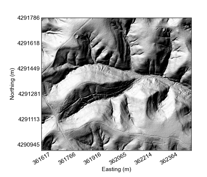
You can also work with the DEM gabilan.bil that is included by default in the /LSDTopoTools/Topographic_projects/Test_data folder but you will need tochange the parameter files to reflect the different DEM name.
|
7.2. The Channel Extraction tool
Our channel extraction tool bundles four methods of channel extraction. These are:
-
A rudimentary extraction using a drainage area threshold.
-
A geometric method combining elements of the Geonet website[Geonet (Passalacqua et al., 2010) and Pelletier (2013) methods that we developed for Grieve et al. (2016) and Clubb et al. (2016) We call this the "Wiener" method (after the wiener filter used to preprocess the data).
These methods are run based on a common interface via the program channel_extraction_tool.exe.
7.3. Running channel extraction with a parameterfile
We assume you have compiled the channel extraction tool (if not, go back here).
Like most of LSDTopoTools, you run this program by directing it to a parameter file. The parameter file has a series of keywords. Our convention is to place the parameter file in the same directory as your data.
7.3.1. Channel extraction options
The parameter file has keywords followed by a value. The format of this file is similar to the files used in the LSDTT_analysis_from_paramfile program, which you can read about in the section Running your first analysis.
The parameter file has a specific format, but the filename can be anything you want. We tend to use the extensions .param and .driver for these files, but you could use the extension .MyDogSpot if that tickled your fancy.
|
The parameter file has keywords followed by the : character. After that there is a space and the value.
Below are options for the parameter files. Note that all DEMs must be in ENVI bil format (DO NOT use ArcMap’s bil format: these are two different things. See the section What data does LSDTopoToolbox take? if you want more details).
The reason we use bil format is because it retains georeferencing which is essential to our file output since many of the files output to csv format with latitude and longitude as coordinates.
| Keyword | Input type | Description |
|---|---|---|
write path |
string |
The path to which data is written. The code will NOT create a path: you need to make the write path before you start running the program. |
read path |
string |
The path from which data is read. |
write fname |
string |
The prefix of rasters to be written without extension.
For example if this is |
read fname |
string |
The filename of the raster to be read without extension. For example if the raster is |
channel heads fname |
string |
The filename of a channel heads file. You can import channel heads. If this is set to |
| Keyword | Input type | Default value | Description |
|---|---|---|---|
print_area_threshold_channels |
bool |
true |
Calculate channels based on an area threshold. |
print_dreich_channels |
bool |
false |
Calculate channels based on the dreich algorithm. |
print_pelletier_channels |
bool |
false |
Calculate channels based on the pelletier algorithm. |
print_wiener_channels |
bool |
false |
Calculate channels based on our wiener algorithm. |
| Keyword | Input type | Default value | Description |
|---|---|---|---|
print_stream_order_raster |
bool |
false |
Prints a raster with channels indicated by their strahler order and nodata elsewhere. File includes "_SO" in the filename. |
print_channels_to_csv |
bool |
true |
Prints a csv file with the channels, their channel pixel locations indicated with latitude and longitude in WGS84. |
print_sources_to_raster |
bool |
false |
Prints a raster with source pixels indicated. |
print_sources_to_csv |
bool |
true |
Prints a csv file with the sources, their locations indicated with latitude and longitude in WGS84. |
print_fill_raster |
bool |
false |
Prints the fill raster |
write hillshade |
bool |
false |
Prints the hillshade raster to file (with "_hs" in the filename). |
print_wiener_filtered_raster |
bool |
false |
Prints the raster after being filter5ed by the wiener filter to file. |
print_curvature_raster |
bool |
false |
Prints two rasters of tangential curvature. One is short and one long wave (has "_LW" in name) curvature. |
| Keyword | Input type | Default value | Description |
|---|---|---|---|
min_slope_for_fill |
float |
0.0001 |
Minimum slope between pixels used by the filling algorithm. |
surface_fitting_radius |
float |
6 |
Radius of the polyfit window over which to calculate slope and curvature. |
curvature_threshold |
float |
0.01 |
Threshold curvature for channel extraction. Used by Pelletier (2013) algorithm. |
minimum_drainage_area |
float |
400 |
Used by Pelletier (2013) algorithm as the minimum drainage area to define a channel. In m2 |
pruning_drainage_area |
float |
1000 |
Used by the wiener and driech methods to prune the drainage network. In m2 |
threshold_contributing_pixels |
int |
1000 |
Used to establish an initial test network, and also used to create final network by the area threshold method. |
connected_components_threshold |
int |
100 |
Minimum number of connected pixels to create a channel. |
A_0 |
float |
1 |
The A0 parameter (which nondimensionalises area) for chi analysis. This is in m2. Used by Dreich. |
m_over_n |
float |
0.5 |
The m/n paramater (sometimes known as the concavity index) for calculating chi. Used only by Dreich. |
number_of_junctions_dreich |
int |
1 |
Number of tributary junctions downstream of valley head on which to run DrEICH algorithm. |
7.3.2. Example channel extraction parameter file
Below is an exaple parameter file. This file is included in the repository along with the driver functions.
# Parameters for channel extraction
# Comments are preceeded by the hash symbol
# Documentation can be found here:
# TBA
# These are parameters for the file i/o
# IMPORTANT: You MUST make the write directory: the code will not work if it doens't exist.
read path: /LSDTopoTools/Topographic_projects/test_data
write path: /LSDTopoTools/Topographic_projects/test_data
read fname: gabilan
write fname: gabilan
channel heads fname: NULL
# Parameter for filling the DEM
min_slope_for_fill: 0.0001
# Parameters for selecting channels and basins
# threshold_contributing_pixels: 2500
print_area_threshold_channels: false
print_wiener_channels: false
print_pelletier_channels: false
print_dreich_channels: true
# write hillshade: true
print_stream_order_raster: true7.4. Channel extraction using thresholds
One of the simplest ways of extracting channel networks from DEMs uses a contributing area threshold. This method is useful for coarse resolution (e.g. >10m) DEMs, where topographic features of the channel heads themselves cannot be reliably identified from the DEM. The user has to specify the threshold area, which represents the upstream area that must drain to a pixel before it is considered as part of the channel.
| The area threshold chosen will affect the density of the channel network. This should be considered carefully, and compared against field-mapped channel head data if these are available. |
7.4.1. Extracting the network with an area threshold using the Channel extraction tool
-
To extract a network using a threshold area, you need to switch on the
print_area_threshold_channelsoption. -
The parameter file will look something like this:
# Parameters for channel extraction # Comments are preceeded by the hash symbol # Documentation can be found here: # TBA # These are parameters for the file i/o # IMPORTANT: You MUST make the write directory: the code will not work if it doens't exist. read path: /LSDTopoTools/Topographic_projects/test_data write path: /LSDTopoTools/Topographic_projects/test_data read fname: gabilan write fname: gabilan channel heads fname: NULL # Parameter for filling the DEM min_slope_for_fill: 0.0001 # Parameters for selecting channels and basins threshold_contributing_pixels: 2500 print_area_threshold_channels: true # Printing of the data write hillshade: true print_stream_order_raster: true print_channels_to_csv: true -
Save this parameter file in the directory with the data (i.e., in
/LSDTopoTools/Topographic_projects/test_data). Call it something sensible. -
Now got into the directory with the chi mapping tool (i.e.,
/LSDTopoTools/Git_projects/LSDTopoTools_ChannelExtraction/driver_functions_ChannelExtraction) and run:$ ./chi_mapping_tool.exe /LSDTopoTools/Topographic_projects/test_data NAME_OF_PARAMFILE.driver -
This should print out both a raster of stream orders and a hillshade raster, and in addition a
csvfile with channel nodes. If you import thiscsvinto a GIS you should select the coordinate system WGS84.
7.4.2. Basic channel extraction using thresholds (the old way)
One of the simplest ways of extracting channel networks from DEMs uses a contributing area threshold. This method is useful for coarse resolution (e.g. >10m) DEMs, where topographic features of the channel heads themselves cannot be reliably identified from the DEM. The user has to specify the threshold area, which represents the upstream area that must drain to a pixel before it is considered as part of the channel.
| The area threshold chosen will affect the density of the channel network. This should be considered carefully, and compared against field-mapped channel head data if these are available. |
We will work through an example using the Indian Creek example dataset that you downloaded.
Compile the code
We can extract threshold area channel networks using the driver function called channel_extraction_area_threshold.cpp. To compile the code you first need to navigate to the driver functions folder in the repository.
$ cd driver_functions_ChannelExtraction/When in this folder type the following to compile the driver:
$ make -f channel_extraction_area_threshold.makeThis will create a program called channel_extraction_area_threshold.out
Run the analysis
To run the analysis you first need to create a parameter file, with which we will set the key user-defined parameters. To create your parameter file, open any text editor and create a file with the following lines:
Name of the DEM without extension
Minimum slope for filling the DEM (suggested to be 0.0001)
Threshold area for channel extractionThe threshold area must be given in m2. You need to save this parameter file in the folder LSDTopoTools_ChannelExtraction (one folder above the driver functions folder). For the Indian Creek site we can create a parameter file called indian_creek_threshold.driver with the following lines:
indian_creek
0.0001
1000After creating the parameter file we can then run the code using the following command:
$ ./channel_extraction_area_threshold.out /path_to_repository_folder/ param_file_nameFor our Indian Creek example our command would be:
$ ./channel_extraction_area_threshold.out /home/LSDTT_repositories/LSDTopoTools_ChannelExtraction/ indian_creek_threshold.driverOnce this program has run, it will create several files with the extracted channel network. These include:
-
A CSV file with the channel heads e.g.
indian_creek_CH_nodeindices_for_arc.csv -
A
bilfile with the channel heads e.g.indian_creek_CH.bil -
A
bilfile with the stream network with Strahler stream ordering e.g.indian_creek_SO.bil
The figure below shows the extracted channel network for the Indian Creek field site with a threshold of 1000 m2.
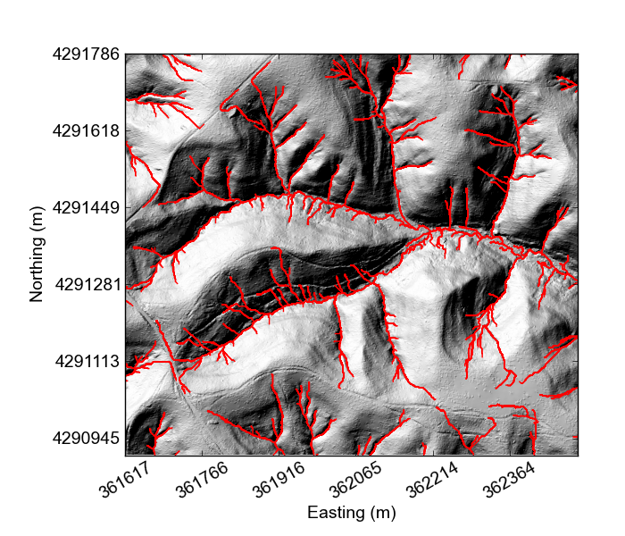
7.5. Geometric channel extraction method
For higher-resolution DEMs a number of different methods have been developed to extract channel networks more accurately. This section details how to extract channels using methods relying on geometric signatures of channel incision, primarily how it affects planform curvature. Although many methods have been developed that use a variety of planform curvature to detect channel heads, we will discuss three methods: the Geonet method the Geonet method (developed by Passalacqua et al. 2010a, b, 2012), a method developed by Pelletier (2013) and implemented in LSDTopoTools, and a similar geometric method available within LSDTopoTools.
To run the Dreich algorithm you need to have the Fast Fourier Transform Library downloaded into your folder LSDTopoTools_ChannelExtraction. You can download it at http://www.fftw.org/download.html. If you are using vagrant this will already be installed, so you can ignore this message.
|
7.5.1. Extracting the network with geometric methods using the Channel extraction tool
-
The Channel extraction tool has two "geometric" channel extraction options.
-
To extract a network using the Pelletier methods, you need to switch on the
print_pelletier_channelsoption. -
To extract a network using the LSDTopoTools Wiener filter method, you need to switch on the
print_wiener_channelsoption. This method was used by Grieve et al., ESURF, 2016 in an attempt to balance what we feel are the strongest components of the Pelletier (2013) and Geonet (by Passalacqua et al) methods.
-
-
The parameter file will look something like this:
# Parameters for channel extraction # Comments are preceeded by the hash symbol # These are parameters for the file i/o # IMPORTANT: You MUST make the write directory: the code will not work if it doens't exist. read path: /LSDTopoTools/Topographic_projects/test_data write path: /LSDTopoTools/Topographic_projects/test_data read fname: gabilan write fname: gabilan channel heads fname: NULL # Parameter for filling the DEM min_slope_for_fill: 0.0001 # Parameters for selecting channels and basins threshold_contributing_pixels: 1000 print_pelletier_channels: true print_wiener_channels: true # Printing of the data write hillshade: true print_stream_order_raster: true print_channels_to_csv: true -
In the above parameter file, I’ve used mostly defaults, with the exception of
print_dreich_channels: true. -
Save this parameter file in the directory with the data (i.e., in
/LSDTopoTools/Topographic_projects/test_data). Call it something sensible. -
Now got into the directory with the chi mapping tool (i.e.,
/LSDTopoTools/Git_projects/LSDTopoTools_ChannelExtraction/driver_functions_ChannelExtraction) and run:$ ./chi_mapping_tool.exe /LSDTopoTools/Topographic_projects/test_data NAME_OF_PARAMFILE.driver -
This should print out both a raster of stream orders and a hillshade raster, and in addition a
csvfile with channel nodes. If you import thiscsvinto a GIS you should select the coordinate system WGS84.
7.5.2. Geometric channel extraction methods (the old way)
For higher-resolution DEMs a number of different methods have been developed to extract channel networks more accurately. This section details how to extract channels using methods relying on geometric signatures of channel incision, primarily how it affects planform curvature. Although many methods have been developed that use a variety of planform curvature to detect channel heads, we will discuss three methods: the Geonet method the Geonet method (developed by Passalacqua et al. 2010a, b, 2012), a method developed by Pelletier (2013) and implemented in LSDTopoTools, and a similar geometric method available within LSDTopoTools.
Geonet (external software)
The Geonet algorithm filters the DEM using a Perona-Malik filter, then uses a planform curvature threshold which is statistically derived from the landscape to detect channel heads. For full information on how Geonet works please see Passalcqua et al. (2010a, b, 2012). It then uses a contributing area threshold to thin the skeleton and create the final channel network. The Geonet algorithm is available free to download from the Geonet website. This site also contains the code documentation and user guides on how to get started with Geonet. It is a cross platform MATLAB package (you will need a MATLAB licence to run in its present form).
Pelletier
Pelletier (2013) developed an algorithm that is similar to Geonet in that it identifies channel heads based on a planform curvature threshold. The main differences between this algorithm and Geonet are:
-
It uses an optimal Wiener threshold to filter the data rather than a Perona-Malik filter
-
It sets a user-defined curvature threshold (e.g. 0.1 m-1) rather than defining it statistically for the landscape in question
-
It does not use a contributing area threshold to thin the skeleton - instead it uses a multi-directional flow routing algorithm
The Pelletier algorithm has been implemented in LSDTopoTools. In order to run it you should follow the steps below.
To run the Pelletier algorithm you need to have the Fast Fourier Transform Library downloaded into your folder LSDTopoTools_ChannelExtraction. You can download it at http://www.fftw.org/download.html.
|
Compile the code
To compile the code navigate to the folder driver_functions_ChannelExtraction. In a terminal window type the following to compile the driver:
$ make -f channel_extraction_pelletier.makeThis will create a program called channel_extraction_pelletier.out which you can use to run the code.
Run the analysis
We first need to create a parameter file similar to that for the [Basic channel extraction using thresholds]. To create your parameter file, open any text editor and create a file with the following lines:
Name of the DEM without extension
Minimum slope for filling the DEM (suggested to be 0.0001)
Threshold area for initial channel network (should be small e.g. 250)
Curvature threshold for channel extraction (suggested by Pelletier (2013) to be 0.1 to avoid extracting threshold hillslopes)
Minimum catchment area (suggested to be 400)You need to save this parameter file in the folder LSDTopoTools_ChannelExtraction (one folder above the driver functions folder). For the Indian Creek site we can create a parameter file called indian_creek_pelletier.driver with the following lines:
indian_creek
0.0001
250
0.1
400After creating the parameter file we can then run the code using the following command:
$ ./channel_extraction_pelletier.out /path_to_repository_folder/ param_file_nameFor our Indian Creek example our command would be:
$ ./channel_extraction_pelletier.out /home/LSDTT_repositories/LSDTopoTools_ChannelExtraction/ indian_creek_pelletier.driverOnce this program has run, it will create several files with the extracted channel network. These include:
-
A CSV file with the channel heads e.g.
indian_creek_CH_Pelletier_nodeindices_for_arc.csv -
A
bilfile with the channel heads e.g.indian_creek_CH_Pelletier.bil -
A
bilfile with the stream network with Strahler stream ordering e.g.indian_creek_SO_Pelletier.bil
The figure below shows the extracted channel network using the Pelletier algorithm for the Indian Creek field site with a planform curvature threshold of 0.1 m-1.
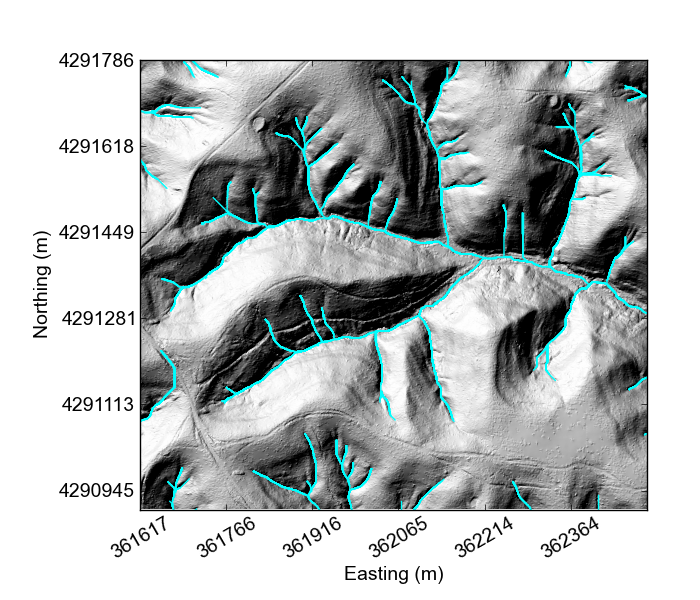
The LSDTopoTools geometric method
Within LSDTopoTools we have also developed a method for extracting channel heads via planform curvature. We first of all filter the DEM using an Optimal Wiener filter, then use a quantile-quantile threshold to statistically determine the planform curvature threshold from the landscape. It then uses a connected components threshold to extract the channel network.
To run the LSDTopoTools algorithm you need to have the Fast Fourier Transform Library downloaded into your folder LSDTopoTools_ChannelExtraction. You can download it at http://www.fftw.org/download.html.
|
Compile the code
To compile the code navigate to the folder driver_functions_ChannelExtraction. In a terminal window type the following to compile the driver:
$ make -f channel_extraction_wiener.makeThis will create a program called channel_extraction_wiener.out which you can use to run the code.
Run the analysis
We first need to create a parameter file similar to that for the [Basic channel extraction using thresholds]. To create your parameter file, open any text editor and create a file with the following lines:
Path and file name of the DEM without extension
Path and output name prefix for your files
Path and output name prefix for the quantile-quantile information
Window radius for filtering the DEM
Threshold area for thinning the channel skeleton
Connected components threshold (should be 100)The threshold area is given in m2. You need to save this parameter file in the folder LSDTopoTools_ChannelExtraction (one folder above the driver functions folder). For the Indian Creek site we can create a parameter file called indian_creek_wiener.driver with the following lines:
RasterFile /home/LSDTT_repositories/LSDTopoTools_ChannelExtraction/indian_creek
OutputRasterFile /home/LSDTT_repositories/LSDTopoTools_ChannelExtraction/indian_creek
QQFile /home/LSDTT_repositories/LSDTopoTools_ChannelExtraction/indian_creek_qq
window_radius_for_surface_fitting 6
threshold_drainage_area 1000
connected_components_threshold 100After creating the parameter file we can then run the code using the following command:
$ ./channel_extraction_wiener.out /path_to_repository_folder/ param_file_nameFor our Indian Creek example our command would be:
$ ./channel_extraction_wiener.out /home/LSDTT_repositories/LSDTopoTools_ChannelExtraction/ indian_creek_wiener.driverOnce this program has run, it will create several files with the extracted channel network. These include:
-
A CSV file with the channel heads e.g.
indian_creek_CH_wiener_nodeindices_for_arc.csv -
A
bilfile with the channel heads e.g.indian_creek_CH_wiener.bil -
A
bilfile with the stream network with Strahler stream ordering e.g.indian_creek_SO_wiener.bil
The figure below shows the extracted channel network using the LSDTopoTools geometric algorithm with an Optimal Wiener filter for the Indian Creek field site.
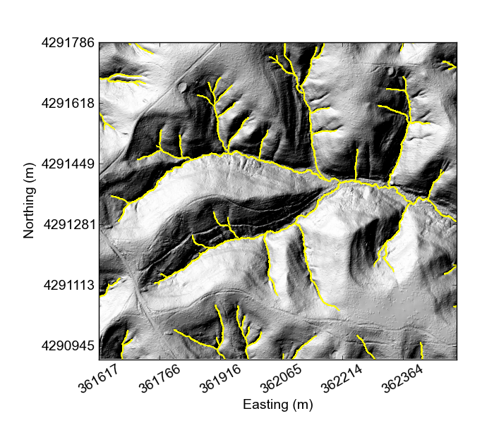
7.6. Channel extraction using the Driech method
The Dreich method of channel head extraction aims to find channel heads by looking at the break in the properties of topographic profiles that occur when fluvial incision gives way to hillslope sediment transport processes. It is different from the geometric methods described above in that it looks for a theoretical signal of fluvial incision rather than the planform curvature of the landscape. The method you use should be chosen based on the particular aims of your study: if you are interested in extracting the valley network (all concave parts of the landscape) then you should use a geometric method, but if you are interested in extracting the fluvial channel network then you should use the Dreich method.
The stable version of the Dreich algorithm that was released with our WRR paper is hosted on CSDMS. The version available from our GitHub repository is the newest version of the code containing some improvements over the stable version. We have made some changes to the way that valleys are extracted from the DEM before the Dreich algorithm is run. In our previous version we used a curvature threshold of 0.1 m-1 to select valleys for analysis as a pre-processing stage. We have now changed the code so that this curvature threshold is statistically derived from the landscape in question using the same method as that of the Geonet algorithm (Passalacqua et al., 2010a, b, 2012). After the initial valley network is extracted, the user may then select the stream order of valleys in which to run the DrEICH algorithm.
To run the Dreich algorithm you need to have the Fast Fourier Transform Library downloaded into your folder LSDTopoTools_ChannelExtraction. You can download it at http://www.fftw.org/download.html. If you are using vagrant this will already be installed, so you can ignore this message.
|
7.6.1. Extracting the network with the Driech method using the Channel extraction tool
-
To extract a network using the DrEICH method, you need to switch on the
print_dreich_channelsoption. -
The parameter file will look something like this:
# Parameters for channel extraction # Comments are preceeded by the hash symbol # These are parameters for the file i/o # IMPORTANT: You MUST make the write directory: the code will not work if it doens't exist. read path: /LSDTopoTools/Topographic_projects/test_data write path: /LSDTopoTools/Topographic_projects/test_data read fname: gabilan write fname: gabilan channel heads fname: NULL # Parameter for filling the DEM min_slope_for_fill: 0.0001 # Parameters for selecting channels and basins threshold_contributing_pixels: 1000 print_dreich_channels: true surface_fitting_radius: 6 number_of_junctions_dreich: 1 connected_components_threshold: 100 m_over_n: 0.5 # Printing of the data write hillshade: true print_stream_order_raster: true print_channels_to_csv: true -
In the above parameter file, I’ve used mostly defaults, with the exception of
print_dreich_channels: true. -
Save this parameter file in the directory with the data (i.e., in
/LSDTopoTools/Topographic_projects/test_data). Call it something sensible. -
Now got into the directory with the chi mapping tool (i.e.,
/LSDTopoTools/Git_projects/LSDTopoTools_ChannelExtraction/driver_functions_ChannelExtraction) and run:$ ./chi_mapping_tool.exe /LSDTopoTools/Topographic_projects/test_data NAME_OF_PARAMFILE.driver -
This should print out both a raster of stream orders and a hillshade raster, and in addition a
csvfile with channel nodes. If you import thiscsvinto a GIS you should select the coordinate system WGS84.
7.6.2. Channel extraction using the Dreich method (the old way)
Run the chi analysis
Before the Dreich algorithm can be run the m/n value for the landscape must be determined. This can be done using the Chi analysis in LSDTopoTools.
Compile the code
We can extract threshold area channel networks using the driver function called channel_extraction_dreich.cpp. To compile the code you first need to navigate to the driver functions folder in the repository. When in this folder type the following to compile the driver:
$ make -f channel_extraction_dreich.makeThis will create a program called channel_extraction_dreich.out
Run the analysis
We first need to create a parameter file similar to that for the [Basic channel extraction using thresholds]. To create your parameter file, open any text editor and create a file with the following lines:
Path and file name of the DEM without extension
Path and output name prefix for your files
Window radius for filtering the DEM
Threshold area for initial channel network (should be 1000)
Connected components threshold for initial valley network (should be 100)
A_0 for chi analysis (should be 1000)
m/n value for landscape (calculate using Chi analysis tools)
Number of tributary junctions downstream of valley head to run DrEICH algorithm on (set to 1 for whole valley network)You need to save this parameter file in the folder LSDTopoTools_ChannelExtraction (one folder above the driver functions folder). For the Indian Creek site we can create a parameter file called indian_creek_dreich.driver with the following lines:
RasterFile /home/LSDTT_repositories/LSDTopoTools_ChannelExtraction/indian_creek
OutputRasterFile /home/LSDTT_repositories/LSDTopoTools_ChannelExtraction/indian_creek
window_radius_for_surface_fitting 6
threshold_drainage_area 1000
connected_components_threshold 100
A_0 1000
m_over_n 0.437
number_of_junctions_dreich 1After creating the parameter file we can then run the code using the following command:
$ ./channel_extraction_dreich.out /path_to_repository_folder/ param_file_nameFor our Indian Creek example our command would be:
$ ./channel_extraction_dreich.out /home/LSDTT_repositories/LSDTopoTools_ChannelExtraction/ indian_creek_dreich.driverOnce this program has run, it will create several files with the extracted channel network. These include:
-
A
bilfile with the valley network with Strahler stream ordering e.g.indian_Creek_SO_valley.bil -
A CSV file with the channel heads e.g.
indian_creek_CH_DrEICH_nodeindices_for_arc.csv -
A
bilfile with the channel heads e.g.indian_creek_CH_DrEICH.bil -
A
bilfile with the stream network with Strahler stream ordering e.g.indian_creek_SO_DrEICH.bil
The figure below shows the extracted channel network using the DrEICH algorithm for the Indian Creek field site.
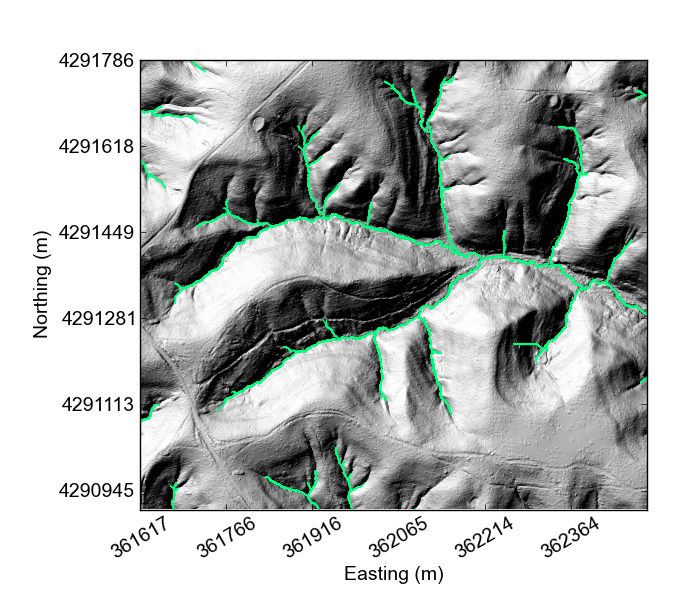
7.7. Summary
By now you should be able to extract channel networks using a variety of methods. For coarse-resolution DEMs you can extract the channel network using a simple area threshold, although the choice of threshold must be carefully considered. For higher-resolution DEMs you can use either a geometric method (if you are interested in extracting the valley network), or a process-based method such as the DrEICH algorithm (if you are interested in the fluvial domain). These methods all require a certain number of user-defined parameters, so the user should take care to select these carefully as their value may impact the resulting channel network.
8. Selecting A Window Size
These instructions will take you through the steps needed to identify the correct window radius to use in the surface fitting routines, following the techniques published in Roering et al. (2010) and Hurst et al. (2012). It is assumed that you are already comfortable with using LSDTopoTools, and have worked though the tutorial: First Analysis. This analysis is often a precursor to other more complex processes, and will ensure that fitted surfaces capture topographic variations at a meaningful geomorphic scale.
8.1. Overview
This driver file will run the surface fitting routines at a range of window sizes up to 100 meters, to produce a series of curvature rasters for the supplied landscape. The mean, interquartile range, and standard deviation of each curvature raster is calculated and these values are written to a text file.
The resulting text file can then be loaded by the provided python script, Window_Size.py,
which will produce plots of how the mean, interquartile range, and standard deviation
of curvature varies with the surface fitting window size.
- This code will produce
-
A
*.txtfile containing the surface statistics for each window size.
8.2. Input Data
This driver only requires an input DEM, this file can be at any resolution and must be
in *.bil, flt or asc. format. Guidance on converting data into these formats
can be found in the chapter covering basic GDAL operations. Note that as data
resolution decreases (i.e. pixel size increases) the ability to resolve individual
hillslopes reduces, and so this technique becomes less important.
8.3. Compile The Driver
The code is compiled using the provided makefile, PolyFitWindowSize.make and the command:
$ make -f PolyFitWindowSize.makeWhich will create the binary file, PolyFitWindowSize.out to be executed.
8.4. Run The Code
The driver is run with three arguments:
- Path
-
The path pointing to where the input raster file is stored. This is also where the output data will be written.
- Filename
-
The filename prefix, without an underscore. If the DEM is called
Oregon_DEM.fltthe filename would beOregon_DEM. This will be used to give the output files a distinct identifier. - Format
-
The input file format. Must be either
bil,fltorasc.
The syntax on a unix machine is as follows:
$ ./PolyFitWindowSize.out <path to data file> <Filename> <file format>And a complete example (your path and filenames may vary):
$ ./PolyFitWindowSize.out /home/s0675405/DataStore/Final_Paper_Data/NC/ NC_DEM flt8.5. The Output Data
The final outputs are stored in a plain text file, <Filename>_Window_Size_Data.txt,
which is written to the data folder supplied as an argument.
This file contains the data needed to select the correct window size. The file has the the following columns, from left to right:
- Length_scale
-
The window size used in the surface fitting routines to generate this row of data.
- Curv_mean
-
Mean curvature for the landscape.
- Curv_stddev
-
Standard deviation of curvature for the landscape.
- Curv_iqr
-
Interquartile range of curvature for the landscape.
8.6. Using Python To Select A Window Size
The latest version of the python scripts which accompany this analysis driver can be found here and provide a complete framework to select a window size for surface fitting.
Once the driver has been run, and the data file, <Filename>_Window_Size_Data.txt,
has been generated, the python script can be executed using:
$ python Window_Size.py <Path> <Data Filename>The two input arguments are similar to the driver file’s inputs:
- Path
-
The full path to where the data file is stored, with a trailing slash. E.g.
/home/data/. This is also where the output plot will be written. - Data Filename
-
The filename of the data file generated by the driver. E.g.
Orgeon_DEM_Window_Size_Data.txt.
A complete example (your path and filenames will be different):
$ python Window_Size.py /home/data/ Oregon_DEM_Window_Size_Data.txtThe plot generated by the python script can be interpreted to select a valid window size for the surface fitting routine. For discussions about this technique refer to Roering et al. (2010) and Hurst et al. (2012). The plot generated should look similar to this example taken from the Gabilan Mesa test dataset, available from the ExampleTopoDatasets repository:
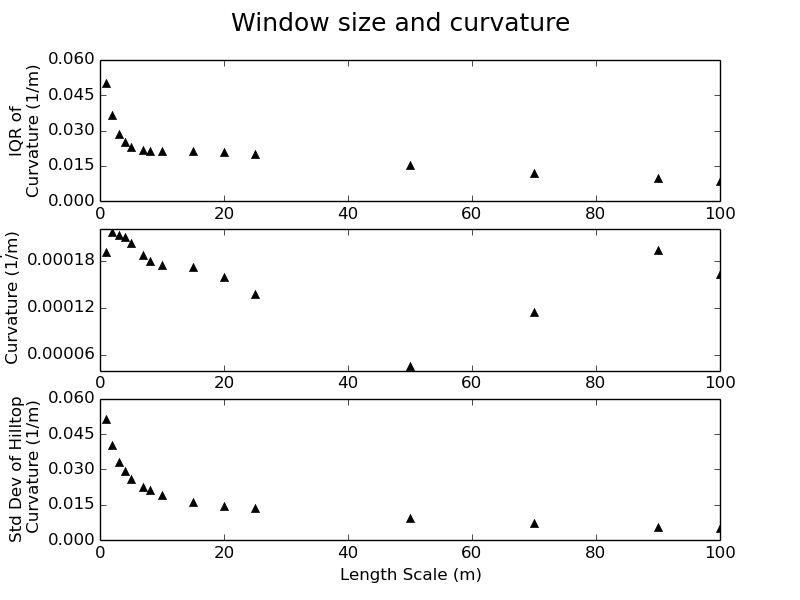
The plot is divided into three sections. The top plot is the change in the interquartile range of curvature with window size, the middle plot is the change in mean curvature with window size and the bottom plot is the change in the standard deviation of curvature with window size.
Roering et al. (2010) and Hurst et al. (2012) suggest that a clear scaling break can be observed in some or all of these three plots, which characterizes the transition from a length scale which captures meter-scale features such as tree throw mounds to a length scale which corresponds to individual hillslopes.
Care must be taken when using this technique as it is challenging to differentiate between measurement noise and topographic roughness (e.g. tree throw mounds) in data if the shot density of the point cloud from which the DEM is generated it too low or it has been poorly gridded. Pay close attention to the metadata provided with your topographic data. If none is provided this is probably a bad sign!
In our example, a length scale of between 4 and 8 meters would be appropriate, supported by the scaling breaks identified in the plots with the red arrows:
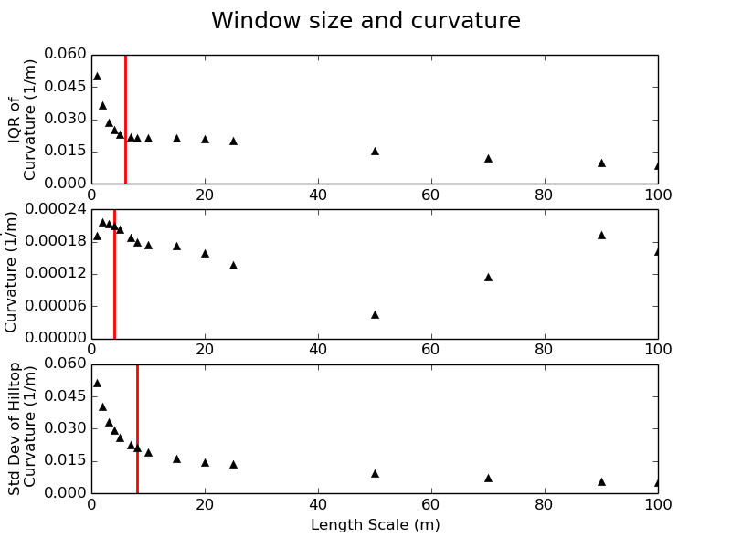
.
9. Extracting Hillslope Lengths
This section gives an overview of how to use the hillslope length driver (LH_Driver.cpp) and it’s companion (LH_Driver_RAW.cpp) to quickly generate hillslope length data for a series of basins, along with other basin average metrics within a larger DEM file. It is assumed that you are already comfortable with using LSDTopoTools, and have worked though the tutorial: First Analysis.
For applications considering landscapes at geomorphic (millenial) timescales use the main
driver, for event scale measurements use the RAW driver. All instructions on this page will
work for either driver. For convenience it will refer only to LH_Driver.cpp but either driver
can be used.
This code is used to to produce the data for Grieve et al. (in review.).
9.1. Overview
This driver file will combine several LSDTopoTools Functions in order to generate as complete a range of basin average and hillslope length metrics as possible. The tool will generate:
-
A HilltopData file with metrics calculated for each hilltop pixel which can be routed to a stream pixel.
-
A file containing basin averaged values of hillslope lengths and other standard metrics.
-
An optional collection of trace files, which can be processed to create a shapefile of the trace paths across the landscape. These can be enabled by setting a flag inside the driver on line 141.
9.2. Input Data
This driver takes the following input data:
| Input data | Input type | Description |
|---|---|---|
Raw DEM |
A raster named |
The raw DEM to be analysed. |
Channel Heads |
Channel head raster named |
A file containing channel heads, which can be generated using the DrEICH algorithm. See the Channel extraction chapter for more information. |
Floodplain Mask |
A binary mask of floodplains named |
Floodplain data which can be used to ensure that analysis only occurs on the hillslopes. This is an optional input. |
Surface Fitting Window Size |
A float |
The surface fitting window size can be constrained using the steps outlined in Selecting A Window Size. This should be performed to ensure the correct parameter values are selected. |
9.3. Compile The Driver
The code is compiled using the provided makefile, LH_Driver.make and the command:
$ make -f LH_Driver.makeWhich will create the binary file, LH_Driver.out to be executed.
9.4. Run The Hillslope Length Driver
The driver is run with six arguments:
- Path
-
The data path where the channel head file and DEM is stored. The output data will be written here too.
- Prefix
-
The filename prefix, without an underscore. If the DEM is called
Oregon_DEM.fltthe prefix would beOregon. This will be used to give the output files a distinct identifier. - Window Size
-
Radius in spatial units of kernel used in surface fitting. Selected using window_size.
- Stream Order
-
The Strahler number of basins to be extracted. Typically a value of 2 or 3 is used, to ensure a good balance between sampling density and basin area.
- Floodplain Switch
-
If a floodplain raster has been generated it can be added to the channel network by setting this switch to
1. This will ensure that hillslope traces terminate at the hillslope-fluvial transition. If no floodplain raster is available, or required, this switch should be set to0. - Write Rasters Switch
-
When running this driver several derivative rasters can be generated to explore the results spatially. If this is required, set this switch to
1. To avoid writing these files set the switch to0. The rasters which will be written are:-
A pit filled DEM
-
Slope
-
Aspect
-
Curvature
-
Stream network
-
Drainage basins of the user defined order
-
Hilltop curvature
-
Hillslope length
-
Hillslope gradient, computed as relief/hillslope length
-
Relief
-
A hillshade of the DEM
-
The syntax to run the driver on a unix machine is as follows:
$ ./LH_Driver.out <Path> <Prefix> <Window Radius> <Stream order> <Floodplain Switch> <Write Rasters Switch>And a complete example (your path and filenames will vary):
$ ./LH_Driver.out /home/s0675405/DataStore/LH_tests/ Oregon 6 2 1 09.5. Analysing The Results
The final outputs are stored in two plain text files, which are written to the data
folder supplied as the argument path.
9.5.1. <Prefix>_Paper_Data.txt
This file contains all of the basin average values for each basin, these files contain a large number of columns, providing a wealth of basin average data. The columns in the file, from left to right are as follows:
-
BasinID = Unique ID for the basin.
-
HFR_mean = Mean hilltop flow routing derived hillslope length.
-
HFR_median = Median hilltop flow routing derived hillslope length.
-
HFR_stddev = Standard deviation of hilltop flow routing derived hillslope length.
-
HFR_stderr = Standard error of hilltop flow routing derived hillslope length.
-
HFR_Nvalues = Number of values used in hilltop flow routing derived hillslope length.
-
HFR_range = Range of hilltop flow routing derived hillslope length.
-
HFR_min = Minimum hilltop flow routing derived hillslope length.
-
HFR_max = Maximum hilltop flow routing derived hillslope length.
-
SA_binned_LH = Hillslope length from binned slope area plot.
-
SA_Spline_LH = Hillslope length from spline curve in slope area plot.
-
LH_Density = Hillslope length from drainage density.
-
Area = Basin area.
-
Basin_Slope_mean = Mean basin slope.
-
Basin_Slope_median = Median basin slope.
-
Basin_Slope_stddev = Standard deviation of basin slope.
-
Basin_Slope_stderr = Standard error of basin slope.
-
Basin_Slope_Nvalues = Number of basin slope values.
-
Basin_Slope_range = Range of basin slopes.
-
Basin_Slope_min = Minimum basin slope.
-
Basin_Slope_max = Maximum basin slope.
-
Basin_elev_mean = Mean basin elevation.
-
Basin_elev_median = Median basin elevation.
-
Basin_elev_stddev = Standard deviation of basin elevation.
-
Basin_elev_stderr = Standard error of basin elevation.
-
Basin_elev_Nvalues = Number of basin elevation values.
-
Basin_elev_Range = Range of basin elevations.
-
Basin_elev_min = Minimum basin elevation.
-
Basin_elev_max = Maximum basin elevation.
-
Aspect_mean = Mean aspect of the basin.
-
CHT_mean = Mean hilltop curvature of the basin.
-
CHT_median = Median hilltop curvature of the basin.
-
CHT_stddev = Standard deviation of hilltop curvature of the basin.
-
CHT_stderr = Standard error of hilltop curvature of the basin.
-
CHT_Nvalues = Number of hilltop curvature values used.
-
CHT_range = Range of hilltop curvatures.
-
CHT_min = Minimum hilltop curvature in the basin.
-
CHT_max = Maximum hilltop curvature in the basin.
-
EStar = \(E*\) value from Roering et al. (2007).
-
RStar = \(R*\) value from Roering et al. (2007).
-
HT_Slope_mean = Mean slope calculated using (relief/hillslope length).
-
HT_Slope_median = Median slope calculated using (relief/hillslope length).
-
HT_Slope_stddev = Standard deviation of slope calculated using (relief/hillslope length).
-
HT_Slope_stderr = Standard error of slope calculated using (relief/hillslope length).
-
HT_Slope_Nvalues = Number of slope values calculated using (relief/hillslope length).
-
HT_Slope_range = Range of slopes calculated using (relief/hillslope length).
-
HT_Slope_min = Minimum slope calculated using (relief/hillslope length).
-
HT_Slope_max = Maximum slope calculated using (relief/hillslope length).
-
HT_relief_mean = Mean relief.
-
HT_relief_median = Median relief.
-
HT_relief_stddev = Standard deviation of relief.
-
HT_relief_stderr = Standard error of relief.
-
HT_relief_Nvalues = Number of relief values used.
-
HT_relief_range = Range of reliefs.
-
HT_relief_min = Minimum relief.
-
HT_relief_max = Maximum relief.
This file can be loaded and the data visualized using these python scripts.
9.5.2. <Prefix>_HilltopData.csv
This file contains hillslope metrics calculated for every hilltop pixel in the dataset which was routed successfully to a stream pixel. The columns in the file, from left to right are as follows:
-
X is the x coordinate of the hilltop pixel.
-
Y is the x coordinate of the hilltop pixel.
-
hilltop_id is the value of the hilltop pixel.
-
S is the slope calculated as relief/hillslope length.
-
R is the relief, the change in elevation between the hilltop and the channel
-
Lh is the hillslope flow length.
-
BasinID is the junction outlet number of the basin the hilltop is within.
-
StreamID is the value of the stream pixel reached by the trace.
-
HilltopSlope is the gradient of the pixel hwere the trace started.
-
DivergentCountFlag is the count of divergent pixels crossed. Depreciated
-
PlanarCountFlag - Count of planar cells crossed Depreciated
-
E_Star = \(E*\) value from Roering et al. (2007).
-
R_Star = \(R*\) value from Roering et al. (2007).
-
EucDist - Euclidean length of the trace from hilltop to channel
This file can be loaded and the data visualized using these python scripts.
9.5.3. Trace Files
An optional switch can be set within the code to print out the coordinates of the path of each trace, allowing hilltop flow paths to be visualized. This option is not exposed at the command line as it will considerably slow the execution of the algorithm.
| This will generate a large number of text files, which some operating systems can struggle to handle. |
To enable this feature open the driver file LH_Driver.cpp and find the following parameters which should be located around line 140:
bool print_paths_switch = false;
int thinning = 1;
string trace_path = "";
bool basin_filter_switch = false;
vector<int> Target_Basin_Vector;These control the path file printing and give several options to limit the scope of the path printing to ensure a manageable number of files are generated. The possible values for each parameter are:
| Parameter | Input type | Description |
|---|---|---|
|
bool |
Set this to |
|
int |
The default value of |
|
string |
The directory that the trace files will be written to, it is strongly recommended that this be an empty directory. |
|
bool |
Set this to |
|
Vector of ints |
If |
Once these parameters have been set, re-compile the driver following the steps in Compile The Driver and run the code. Once the code has executed a large number of files will have been generated in the supplied path. They are plain text, space delimited files which have the following headings:
-
X Coordinate.
-
Y Coordinate.
-
Count of divergent pixels crossed during the trace.
-
Hillslope length.
-
Count of planar pixels crossed during the trace.
-
E_Star from Roering et al. (2007).
-
R_Star from Roering et al. (2007).
-
Euclidean length of trace.
A python script is provided to process these files into a shapefile, which can be viewed in any GIS package, or plotted using other python scripts provided. The python script to process these files is located here and is called trace_process_1_1.py. To run this file, alter the input path to point to where the trace files are stored, and then set the output path to a new directory which must already exist.
The line:
files = files[::100] # only processing every 100th trace for speedis used to thin the dataset to speed up processing, in case this was not performed earlier. Again, a value of 1 will keep all of the data, and any other integer will keep every nth file. Once the code has been executed a single shapefile will be produced in the user defined output directory.
9.6. Worked Example
In this final section a typical hillslope length analysis will be performed from start to finish to demonstrate how to use this algorithm on real data. For this example we will use a very small section of Gabilan Mesa, to facilitate rapid processing.
9.6.1. Getting the data
The data is located in the ExampleTopoDatasets repository. Firstly, we must create a new directory to store our topogrpahic data:
$ mkdir data
$ pwd
/home/s0675405/LH/data/We will only take the data we need, which is the Gabilan Mesa DEM and the associated DrEICH channel head file, so we can use wget to download the data:
$ wget https://github.com/LSDtopotools/ExampleTopoDatasets/raw/master/gabilan.bil
$ wget https://github.com/LSDtopotools/ExampleTopoDatasets/raw/master/gabilan.hdr
$ wget https://github.com/LSDtopotools/ExampleTopoDatasets/raw/master/gabilan_CH.bil
$ wget https://github.com/LSDtopotools/ExampleTopoDatasets/raw/master/gabilan_CH.hdrYou should now have the following files in your data folder:
$ pwd
/home/s0675405/LH/data/
$ ls
gabilan.bil gabilan_CH.bil gabilan_CH.hdr gabilan.hdr9.6.2. Getting The Code
Next we need to download the code from the CSDMS repository where the latest stable version of the hilltop flow routing algorithm is located. This can again be downloaded using wget and it will come as a zipfile, which should be extracted into a separate folder to the data:
$ wget https://github.com/csdms-contrib/Hilltop_flow_routing/archive/master.zip
$ unzip master.zipFinally we need to get the visualization python scripts so we can explore the data:
$ wget https://github.com/sgrieve/LH_Paper_Plotting/archive/master.zip
$ unzip master.zipNow we should have 3 folders, one with the data, one with the main c++ code and a third with the python code.
$ ls
data Hilltop_flow_routing-master LH_Paper_Plotting-master9.6.3. Running The Code
We need to check that the filenames for our input and output data make sense in the LH_Driver.cpp file. Open the file in a text editor and look at the line which loads the DEM:
LSDRaster DEM((path+filename+"_dem"), "flt");We are working with bil files, so need to change the "flt" to "bil", which can be done with a simple search and replace within your text editor.
The code also expects our data to be tagged *_dem so lets rename our data files to make life simpler:
$ pwd
/home/s0675405/LH/data
$ mv gabilan.bil gabilan_dem.bil
$ mv gabilan.hdr gabilan_dem.hdr
$ mv gabilan_CH.bil gabilan_dem_CH.bil
$ mv gabilan_CH.hdr gabilan_dem_CH.hdr
$ ls
gabilan_dem.bil gabilan_dem_CH.bil gabilan_dem_CH.hdr gabilan_dem.hdrNow we can navigate back to the directory where the driver and makefile are stored and make the driver:
$ pwd
/home/s0675405/LH/Hilltop_flow_routing-master/driver_functions_GrieveLH2015
$ make -f LH_Driver.make
g++ -c -Wall -O3 -pg -g ../LSDParticle.cpp -o ../LSDParticle.o
g++ -c -Wall -O3 -pg -g ../LSDCRNParameters.cpp -o ../LSDCRNParameters.o
g++ -Wall -O3 -pg -g LH_Driver.o ../LSDMostLikelyPartitionsFinder.o ../LSDIndexRaster.o ../LSDRaster.o ../LSDFlowInfo.o ../LSDJunctionNetwork.o ../LSDIndexChannel.o ../LSDChannel.o ../LSDStatsTools.o ../LSDBasin.o ../LSDShapeTools.o ../LSDParticle.o ../LSDCRNParameters.o -o LH_Driver.outSome warnings may appear which can be ignored as long as the final few lines look something like they do above and the file LH_Driver.out is created.
The binary file can then be run using the desired input arguments
./LH_Driver.out /home/s0675405/LH/data/ gabilan 5 2 0 0Once the code is completed it will print some data to the screen about the success rate of the traces. Due to the nature of real topography there will always be a small number of failed traces, traces which hit the edge of the DEM should also be rare, but these are excluded from analysis as they are truncated. If these values are very large relative to the stream count, which denotes traces which have successfully completed, there may be a problem with your input data. In the case of this worked example we get the following results:
Hilltop count: 2170
Stream count: 2157
Fail count: 7
Uphill count: 0
Edge count: 6Returning to the data folder we can see the the two data files described earlier in this chapter have been written.
$ pwd
/home/s0675405/LH/data
$ ls
gabilan_dem.bil gabilan_dem_CH.hdr gabilan_dreich__HilltopData.csv
gabilan_dem_CH.bil gabilan_dem.hdr gabilan_dreich_PaperData.txt9.6.4. Plotting Data
We can now load the data files into the python scripts to visualize the data. Firstly, we can make a histogram to view the distribution of hillslope length values for our landscape using the RAW_LH_Hist.py script. We need to update the plotting parameters to reflect our data, the following lines can be edited within the script using any text editor:
#================ modifyable parameters start here ====================
#paths to the data and to save the figure to
path = '../../data/' #path to the folder contaning the hilltopdata files
filename = 'gabilan_dreich__HilltopData.csv'
figpath = path #path to save the final figures
#plot style parameters
xmax = 400
ymax = 40
xstep = 50
ystep = 10
title_move = 0.
#plot labels
location = 'Gabilan Mesa'
#================ modifyable parameters end here ====================The plot style parameters require a bit of trial and error to get the the correct axis limits, so the code may need to be executed several times. Once the parameters have been set the script can be run at the command line:
python RAW_LH_Hist.pyWhich produces a histogram within the data folder.
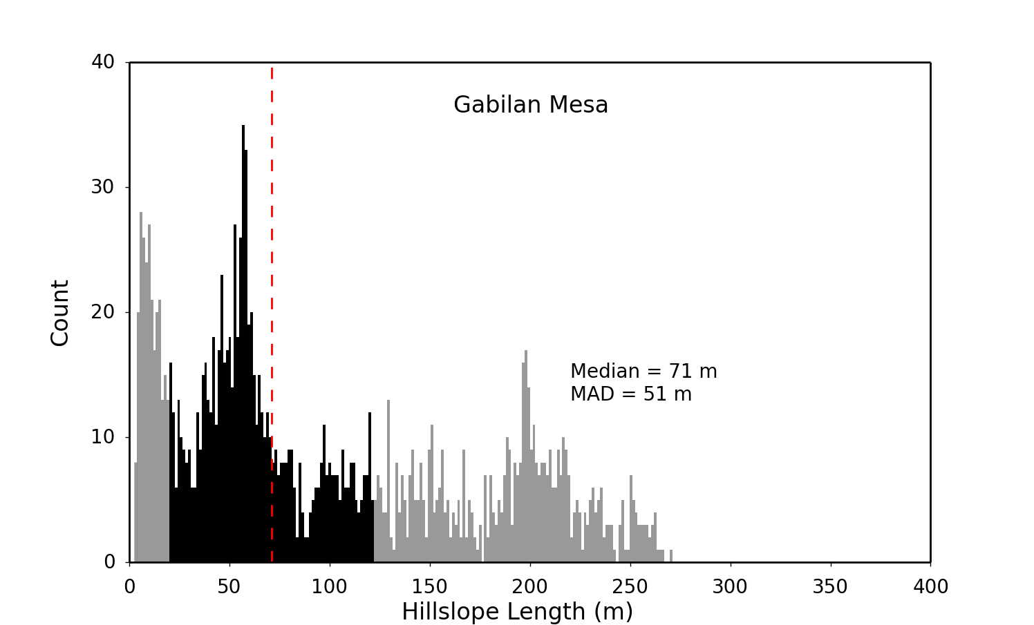
This process can be repeated to run any of the plotting scripts provided with this package, as each has a similar interface.
9.7. Summary
You should now be able to generate hillslope length data from high resolution topography.
10. Dimensionless Erosion and Relief
The relationship between topographic relief and erosion rate can be used to interrogate dynamic forces which interact to shape the Earth’s surface. Roering et al. (2007) formulated a dimensionless relationship between relief (R*) and erosion rate (E*) which allows comparisons between landscapes of vastly differing forms. Hurst et al. (2013) used this technique to identify topographic uplift and decay along the Dragons Back Pressure Ridge, CA. However, in spite of its utility, it has always been a challenging method to implement. In this chapter we go through the steps required to generate E* R* data using LSDTopoTools from high resolution topography at a range of spatial scales, following Grieve et al. (2015).
10.1. Get the code for dimensionless erosion and relief analysis
Our code for E*R* analysis can be found in our GitHub repository. This repository contains code for extracting channel networks, generating hillslope length data and processing this topographic data into a form which can be used to generate E* R* relationships.
10.1.1. Clone the GitHub repository
First navigate to the folder where you will keep the GitHub repository. In this example it is called /home/LSDTT_repositories. To navigate to this folder in a UNIX terminal use the cd command:
$ cd /home/LSDTT_repositories/You can use the command pwd to check you are in the right folder. Once you are in this folder, you can clone the repository from the GitHub website:
$ pwd
/home/LSDTT_repositories/
$ git clone https://github.com/LSDtopotools/LSDTT_Hillslope_Analysis.gitNavigate to this folder again using the cd command:
$ cd LSDTT_Hillslope_Analysis/10.1.2. Alternatively, get the zipped code
If you don’t want to use git, you can download a zipped version of the code:
$ pwd
/home/LSDTT_repositories/
$ wget https://github.com/LSDtopotools/LSDTT_Hillslope_Analysis/archive/master.zip
$ gunzip master.zip
GitHub zips all repositories into a file called master.zip,
so if you previously downloaded a zipper repository this will overwrite it.
|
10.1.3. Get the Python code
In addition to the topographic analysis code, some python code is provided to handle the generation of the E* R* data and its visualization. This code is stored in a separate GitHub repository which can be checked out in the same manner as before. It is a good idea to place the python code into a separate directory to avoid confusion later on.
$ pwd
/home/LSDTT_repositories/
$ git clone https://github.com/sgrieve/ER_Star.gitNavigate to this folder again using the cd command:
$ cd ER_STAR/or if you prefer to avoid git:
$ pwd
/home/LSDTT_repositories/
$ wget https://github.com/LSDtopotools/LSDTopoTools_ER_STAR/archive/master.zip
$ gunzip master.zip| The python code has a number of dependences which you should check prior to trying to run the code, as it could give confusing error messages. |
10.1.4. Checking your Python package versions
For the code to run correctly the following packages must be installed with a version number greater than or equal to the version number listed below. The code has only been tested on Python 2.7 using the listed versions of these packages, so if you experience unexpected behavior on a higher version, try installing the specified version.
- matplotlib
-
Version 1.43
- numpy
-
Verision 1.9.2
- scipy
-
Version 0.16.0
- uncertainties
-
Version 2.4.6
To test if you have a package installed, launch python at the terminal and try to import each package in turn. For example, to test if we have numpy installed:
$ python
Python 2.7.6 (default, Jun 22 2015, 18:00:18)
[GCC 4.8.2] on linux2
Type "help", "copyright", "credits" or "license" for more information.
>>> import numpy
>>>If importing the package does nothing, that means it has worked, and we can now check the version of numpy
>>> numpy.__version__
>>> '1.9.2'In this case my version of numpy is new enough to run Plot_ER_Data.py without any problems. Repeat this test for each of the 4 packages and if any of them are not installed or are too old a version, it can be installed by using pip at the unix terminal or upgraded by using the --upgrade switch.
$ sudo pip install <package name>
$ sudo pip install --upgrade <package name>10.1.5. Get the example datasets
We have provided some example datasets which you can use in order to test this algorithm. In this tutorial we will work using a LiDAR dataset and accompanying channel heads from Gabilan Mesa, California. You can get it from our ExampleTopoDatasets repository using wget and we will store the files in a folder called data:
$ pwd
/home/data
$ wget https://github.com/LSDtopotools/ExampleTopoDatasets/raw/master/gabilan.bil
$ wget https://github.com/LSDtopotools/ExampleTopoDatasets/raw/master/gabilan.hdr
$ wget https://github.com/LSDtopotools/ExampleTopoDatasets/raw/master/gabilan_CH.bil
$ wget https://github.com/LSDtopotools/ExampleTopoDatasets/raw/master/gabilan_CH.hdrThis dataset is already in the preferred format for use with LSDTopoTools (the ENVI bil format). However the filenames are not structured in a manner which the code expects. Both the hillslope length driver and the E*R* driver expect files to follow the format <prefix>_<filetype>.bil so we should rename these four files to follow this format.
$ pwd
/home/so675405/data
$ mv gabilan.bil gabilan_DEM.bil
$ mv gabilan.hdr gabilan_DEM.hdr
$ mv gabilan_CH.bil gabilan_DEM_CH.bil
$ mv gabilan_CH.hdr gabilan_DEM_CH.hdr
$ ls
gabilan_DEM.bil gabilan_DEM_CH.bil gabilan_DEM_CH.hdr gabilan_DEM.hdrNow the prefix for our data is gabilan and we are ready to look at the code itself.
10.2. Processing High Resolution Topography
The generation of E* R* data is built upon the ability to measure hillslope length and relief as spatially continuous variables across a landscape. This is performed by using the hillslope length driver outlined in the Extracting Hillslope Lengths chapter.
When running the hillslope length driver, ensure that the switch to write the rasters is set to 1 as these rasters are required by the E_STAR_R_STAR.cpp driver.
|
This driver performs the hilltop segmentation and data averaging needed to generate E* R* data at the scale of individual hilltop pixels, averaged at the hillslope scale and at a basin average scale.
10.3. Input Data
This driver takes the following input data:
| Input data | Input type | Description |
|---|---|---|
Raw DEM |
A raster named |
The raw DEM to be analysed. |
Hillslope length raster |
A raster named |
A raster of hillslope length measurements generated by |
Topographic relief raster |
A raster named |
A raster of topographic relief measurements generated by |
Hilltop curvature raster |
A raster named |
A raster of hilltop curvature measurements generated by |
Slope raster |
A raster named |
A raster of topographic gradient generated by |
Minimum Patch Area |
An integer |
The minimum number of pixels required for a hilltop to be used for spatial averaging. |
Minimum Number of Basin Data Points |
An integer |
The minimum number of data points required for each basin average value to be computed. |
Basin Order |
An integer |
The Strahler number of basins to be extracted. Typically a value of 2 or 3 is used, to ensure a good balance between sampling density and basin area. |
10.4. Compile The Driver
Once you have generated the hillslope length data you must compile the E_STAR_R_STAR.cpp driver. This is performed by using the provided makefile, LH_Driver.make and the command:
$ make -f E_STAR_R_STAR.makeWhich will create the binary file, E_STAR_R_STAR.out to be executed.
10.5. Run the code
Once the driver has been compiled it can be run using the following arguments:
- Path
-
The data path where the input data files are stored. The output data will be written here too.
- Prefix
-
The filename prefix, without an underscore. If the DEM is called
Oregon_DEM.fltthe prefix would beOregon. This will be used to give the output files a distinct identifier. - Minimum Patch Area
-
The minimum number of pixels required for a hilltop to be used for spatial averaging.
- Minimum Number of Basin Data Points
-
The minimum number of data points required for each basin average value to be computed.
- Basin Order
-
The Strahler number of basins to be extracted. Typically a value of 2 or 3 is used, to ensure a good balance between sampling density and basin area.
In our example we must navigate to the directory where the file was compiled and run the code, providing the five input arguments:
$ pwd
/home/LSDTT_repositories/ER_Code_Package/Drivers
$ ./E_STAR_R_STAR.out /home/data/ gabilan 50 50 2A more general example of the input arguments would is:
$ ./E_STAR_R_STAR.out <path to data files> <filename prefix> <min. patch area> <min. basin pixels> <basin order>Once the code has run, it will produce 5 output files, tagged with the input filename prefix. In the case of our example, these files are:
-
gabilan_E_R_Star_Raw_Data.csv
-
gabilan_E_R_Star_Patch_Data.csv
-
gabilan_E_R_Star_Basin_2_Data.csv
-
gabilan_Patches_CC.bil
-
gabilan_Patches_CC.hdr
The three .csv files are the data files containing the raw, hilltop patch and basin average data which is used by Plot_ER_Data.py to generate the E* R* results. The .bil and accompanying .hdr files contain the hilltop network used for the spatial averaging of the data, with each hilltop coded with a unique ID. This can be used to check the spatial distribution of hilltops across the study site.
10.6. Analyzing Dimensionless Relationships
Once the code has been run and the data has been generated, it can be processed using the Python script Plot_ER_Data.py which was downloaded into the directory:
$ pwd
/home/LSDTT_repositories/ER_Star
$ ls
bin_data.py Plot_ER_Data.py Settings.pyThe three Python files are all needed to perform the E* R* analysis. The main code is contained within Plot_ER_Data.py and it makes use of bin_data.py to perform the binning of the data. The file Settings.py is the file that users should modify to run the code on their data.
Settings.py is a large parameter file which must be modified to reflect our input data and the nature of the plots we want to generate. Each parameter is described within the file, but these descriptions are also produced here for clarity. It should be noted that a useful method for managing large sets of data and plotting permutations is to generate several Settings.py files and swapping between them as needed. The following tables outline all of the parameters which can be used to configure the E* R* plots.
| Parameter Name | Possible Values | Description |
|---|---|---|
Path |
Any valid path |
Must be wrapped in quotes with a trailing slash eg 'home/user/data/' |
Prefix |
Filename prefix |
Must be wrapped in quotes and match the prefix used in |
Order |
Any integer |
Basin order used in |
| Parameter Name | Possible Values | Description |
|---|---|---|
RawFlag |
0 or 1 |
Use 1 to plot the raw data and 0 to not plot it. |
DensityFlag |
Any integer |
Use 0 to not plot the raw data as a density plot and 1 to plot a density plot. Values greater than 1 will be used the thin the data. For example 2 will plot every second point. Reccommended! |
BinFlag |
'raw', 'patches' or '' |
Use 'raw' to bin the raw data, 'patches' to bin the hilltop patch data and an empty string, '' to not perform binning. Note that quotes are needed for all cases. |
NumBins |
Any integer |
Number of bins to be generated. Must be an integer. eg 5,11,20. Will be ignored if |
MinBinSize |
Any integer |
Minimum number of data points required for a bin to be valid. eg 5,20,100. Will be ignored if |
PatchFlag |
0 or 1 |
Use 1 to plot the patch data and 0 to not plot it. |
BasinFlag |
0 or 1 |
Use 1 to plot the basin data and 0 to not plot it. |
LandscapeFlag |
0 or 1 |
Use 1 to plot the landscape average data and 0 to not plot it. |
| Parameter Name | Possible Values | Description |
|---|---|---|
Sc_Method |
A real number or 'raw', 'patches' or 'basins' |
Either input a real number eg 0.8,1.2,1.052 to set the Sc value and avoid the fitting of Sc. Or select 'raw','patches' or 'basins' (including the quotes) to use the named dataset to constrain the best fit Sc value through bootstrapping. |
NumBootsraps |
Any integer |
Number of iterations for the bootstrapping procedure. 10000 is the default, larger values will take longer to process. |
| Parameter Name | Possible Values | Description |
|---|---|---|
ErrorBarFlag |
True or False |
True to plot errorbars on datapoints, False to exclude them. Errorbars are generated as the standard error unless otherwise stated. |
Format |
'png','pdf','ps','eps','svg' |
File format for the output E* R* plots. Must be one of: 'png','pdf','ps','eps','svg', including the quotes. |
GabilanMesa |
True or False |
True to plot the example data from Roering et al. (2007), False to exclude it. |
OregonCoastRange |
True or False |
True to plot the example data from Roering et al. (2007), False to exclude it. |
SierraNevada |
True or False |
True to plot the example data from Hurst et al. (2012), False to exclude it. |
10.6.1. Density Plot
Firstly we will generate a density plot from the raw E* R* data. To do this we must update the path to our data files, the prefix and the basin order so that our files can be loaded. These modifications can be done in any text editor.
As we want to display a density plot we must also place a value other than 0 for the DensityFlag parameter, and ensure that all other parameters in the second parameter table are set to 0 or in the case of BinFlag, an empty string ''.
We will set the critical gradient to a value of 0.8, to avoid running the bootstrapping calculations. ErrorBarFlag should be set to False, along with the example data options, and the file format can be left as the default value.
The below complete settings file has the comments removed for clarity, as these are not needed by the program.
# Parameters to load the data
Path = '/home/s0675405/data/'
Prefix = 'gabilan'
Order = 2
# Options to select data to be plotted
RawFlag = 0
DensityFlag = 1
BinFlag = ''
NumBins = 20
MinBinSize = 100
PatchFlag = 0
BasinFlag = 0
LandscapeFlag = 0
# Options regarding the fitting of the critical gradient
Sc_Method = 0.8
NumBootsraps = 100
# Plot style options
ErrorBarFlag = False
Format = 'png'
# Comparison data to be plotted from the other studies
GabilanMesa = False
OregonCoastRange = False
SierraNevada = FalseOnce the settings file has been generated, the code can be run from the terminal:
$ python Plot_ER_Data.pyThis will write a file called gabilan_E_R_Star.png to the data folder, which should look like this:
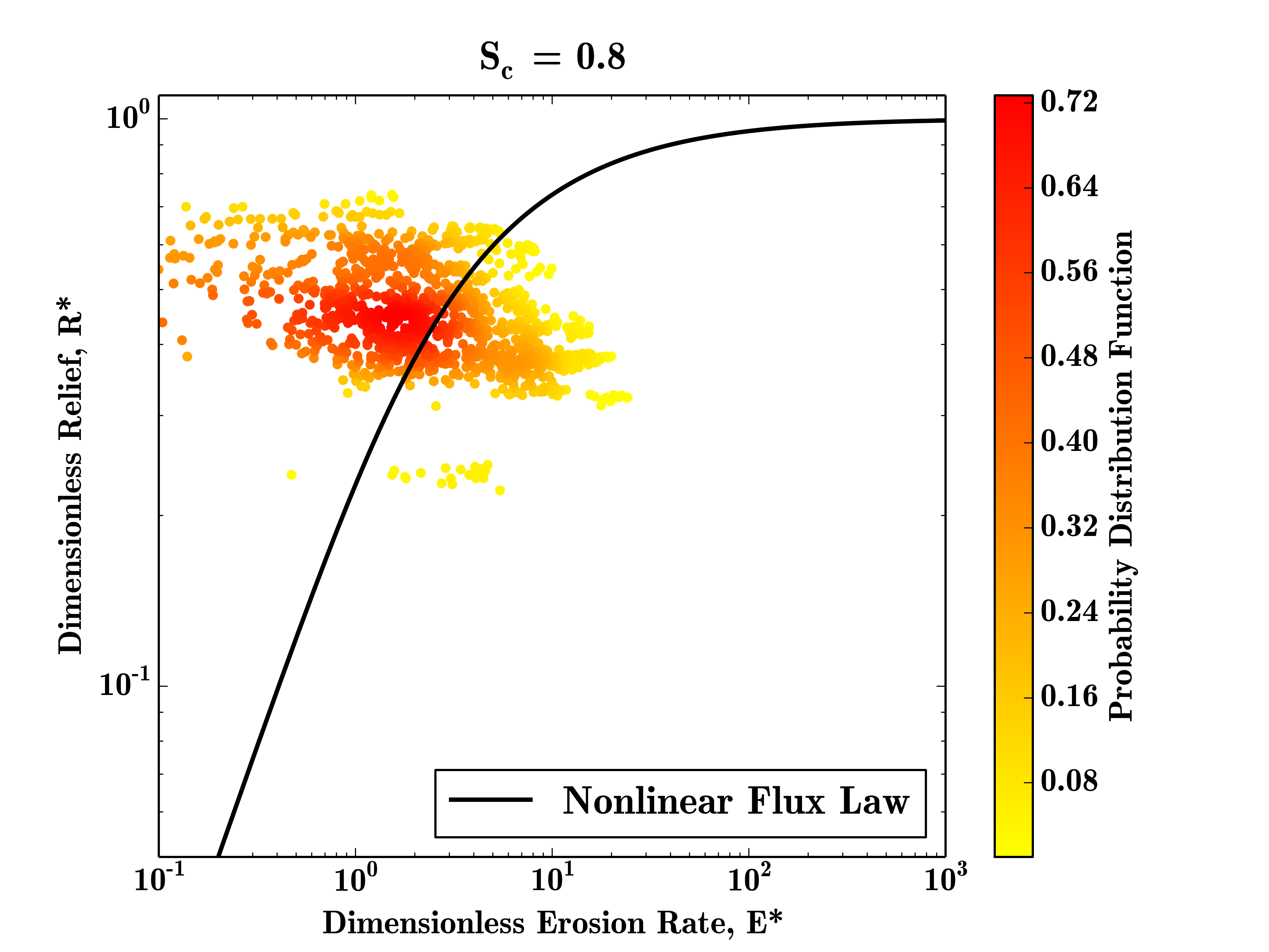
This plot shows the density of the E* R* measurements for this test datatset, the data is quite sparse due to the small size of the input DEM, but the majority of data points still plot close to the steady state curve.
10.6.2. Hilltop Patch Plot
Having completed the first example plot it becomes very simple to re-run the code to generate different plots. In this example we will plot the hilltop patch data points with error bars. To do this we need to change our settings file as follows:
# Parameters to load the data
Path = '/home/s0675405/data/'
Prefix = 'gabilan'
Order = 2
# Options to select data to be plotted
RawFlag = 0
DensityFlag = 0
BinFlag = ''
NumBins = 20
MinBinSize = 100
PatchFlag = 1
BasinFlag = 0
LandscapeFlag = 0
# Options regarding the fitting of the critical gradient
Sc_Method = 0.8
NumBootsraps = 100
# Plot style options
ErrorBarFlag = True
Format = 'png'
# Comparison data to be plotted from the other studies
GabilanMesa = False
OregonCoastRange = False
SierraNevada = FalseThis set of parameters generates a small number of hilltop patch data points which plot in similar locations as the raw data.
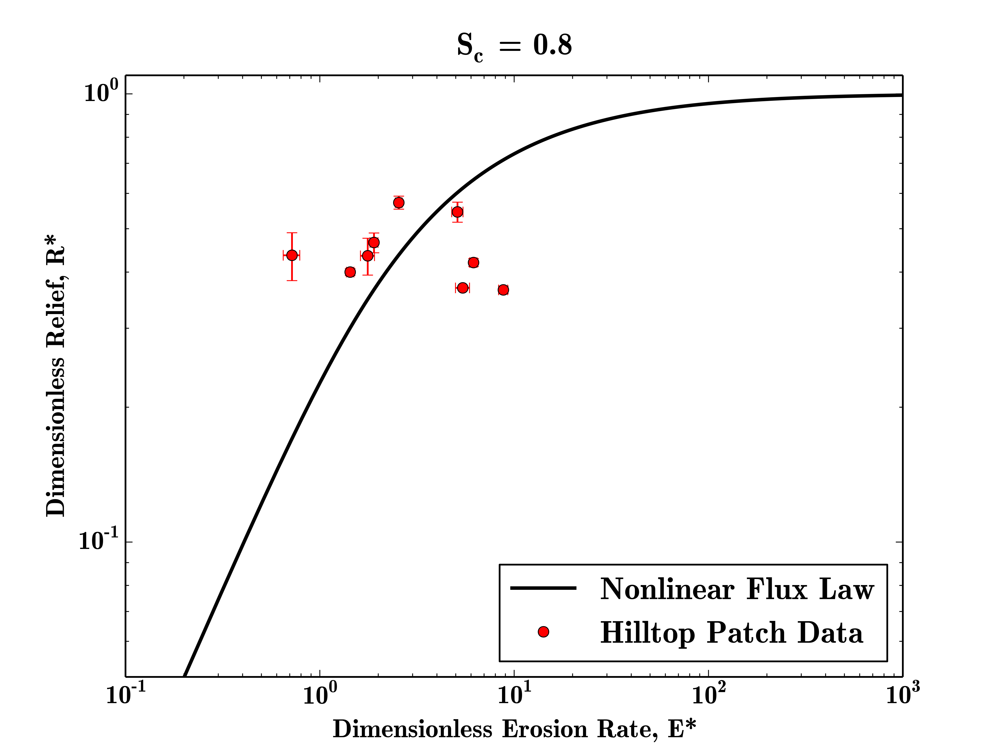
To plot the basin average data, the same set of paramters would be used
10.6.3. Binned Plot
To bin the raw data, we need to set the BinFlag parameter to 'raw' and select a number of bins to place our data into:
# Parameters to load the data
Path = '/home/s0675405/data/'
Prefix = 'gabilan'
Order = 2
# Options to select data to be plotted
RawFlag = 0
DensityFlag = 0
BinFlag = 'raw'
NumBins = 20
MinBinSize = 100
PatchFlag = 0
BasinFlag = 0
LandscapeFlag = 0
# Options regarding the fitting of the critical gradient
Sc_Method = 0.8
NumBootsraps = 100
# Plot style options
ErrorBarFlag = True
Format = 'png'
# Comparison data to be plotted from the other studies
GabilanMesa = False
OregonCoastRange = False
SierraNevada = FalseIn this case, the result is fairly meaningless, as most of the bins have too few data points to be plottted, but on larger datasets this method can highlight landscape transience very clearly.
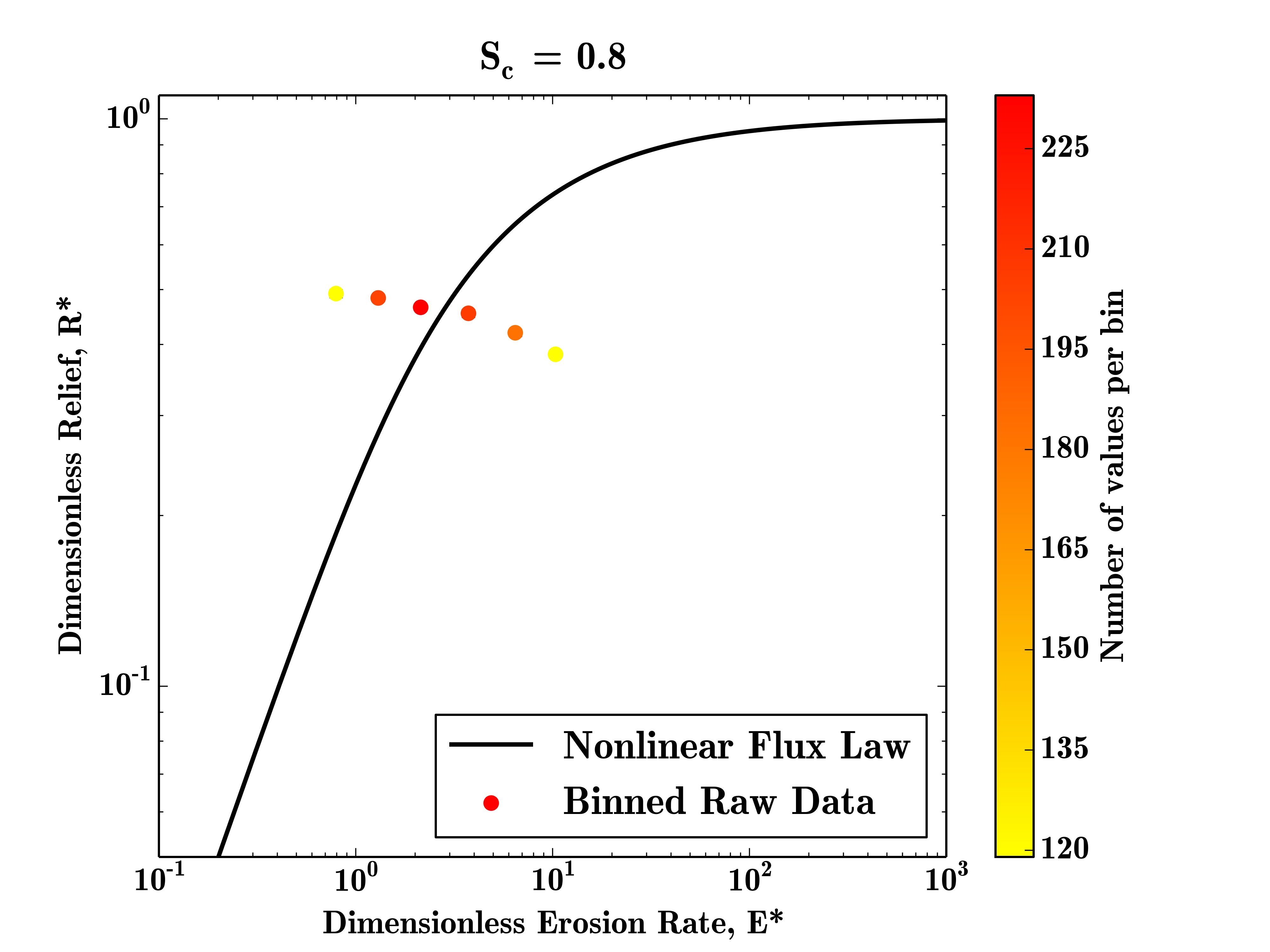
10.6.4. Fitting The Critical Gradient
The final example for this section is how to use the code to estimate the critical gradient of a landscape. This is performed by configuring the bootstrapping parameters and in this case we will use the patch data and 1000 iterations to compute the best fit critical gradient.
# Parameters to load the data
Path = '/home/s0675405/data/'
Prefix = 'gabilan'
Order = 2
# Options to select data to be plotted
RawFlag = 0
DensityFlag = 0
BinFlag = ''
NumBins = 20
MinBinSize = 100
PatchFlag = 1
BasinFlag = 0
LandscapeFlag = 0
# Options regarding the fitting of the critical gradient
Sc_Method = 'patches'
NumBootsraps = 1000
# Plot style options
ErrorBarFlag = True
Format = 'png'
# Comparison data to be plotted from the other studies
GabilanMesa = False
OregonCoastRange = False
SierraNevada = FalseIt should be noted that on a small dataset such as this the fitting will not be very robust as there are too few data points, but this example should demonstrate how to run the code in this manner on real data. The best fit critical gradient will be printed at the top of the final plot.
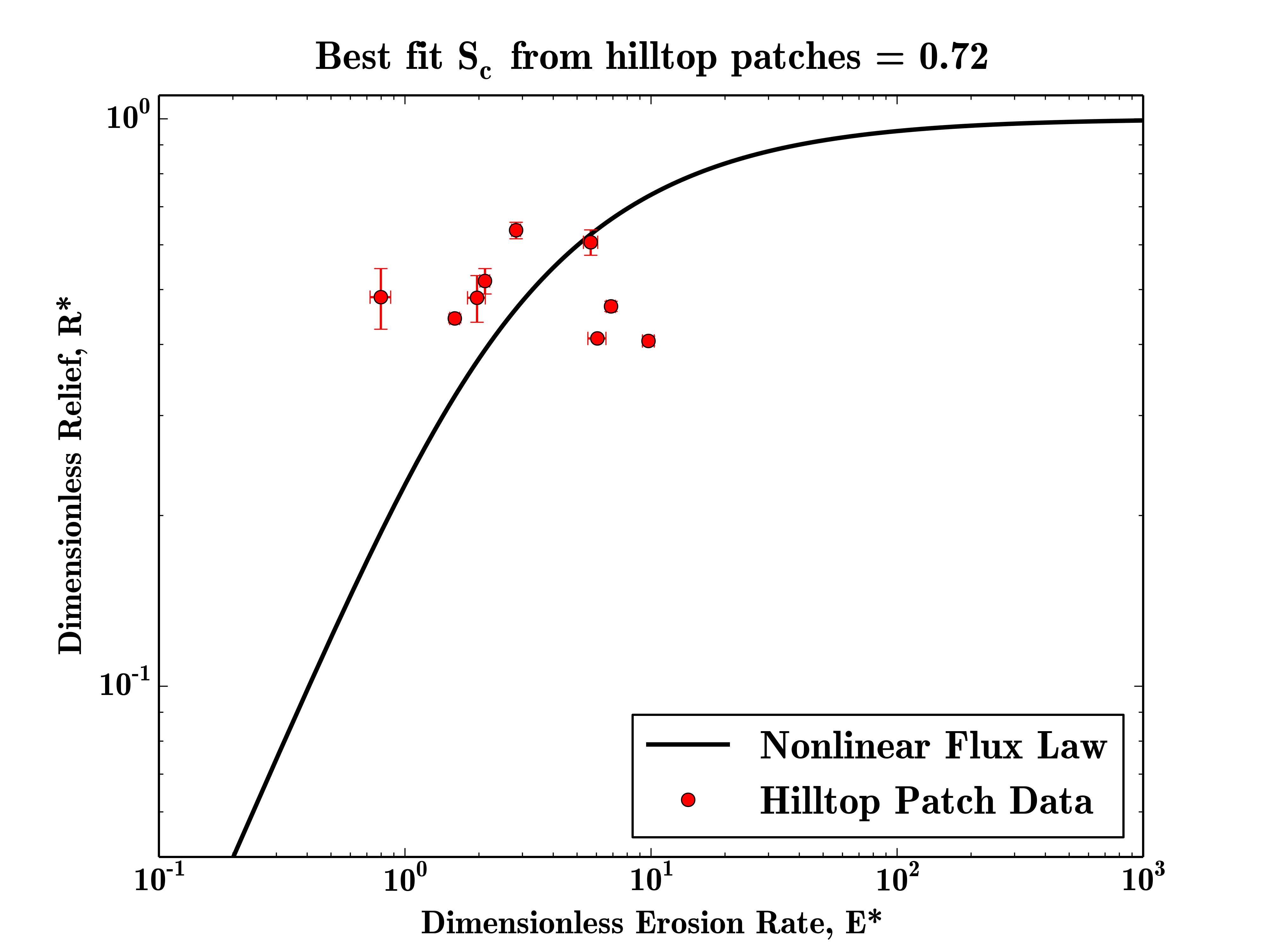
10.7. Summary
By now you should be able to generate dimensionless erosion rate and relief data from high resolution topography.
11. Chi analysis
In the late 1800s, G.K. Gilbert proposed that bedrock channel incision should be proportional to topographic gradients and the amount of water flowing in a channel.
We have already seen that erosion is favored by declivity. Where the declivity is great the agents of erosion are powerful; where it is small they are weak; where there is no declivity they are powerless. Moreover it has been shown that their power increases with the declivity in more than simple ratio.
Geology of the Henry Mountains 1877
Since then, many geomorpholgists have attempted to extract information about erosion rates from channel profiles. Chi analysis is a method of extracting information from channel profiles that attempts to compare channels with different discharges first proposed by Leigh Royden and colleagues at MIT. LSDTopoTools has a number of tools for performing chi analysis.
This document gives instructions on how to use the segment fitting tool for channel profile analysis developed by the Land Surface Dynamics group at the University of Edinburgh. The tool is used to examine the geometry of channels using the integral method of channel profile analysis. For background to the method, and a description of the algorithms, we refer the reader to Mudd et al. (2014). For background into the strengths of the integral method of channel profile analysis, the user should read Perron and Royden (2013, ESPL).
This document guides the user through the installation process, and explains how to use the model.
You will need a C++ compiler for this tutorial. If you have no idea what a C++ compiler is, see the appendix.
Visualisation of the model results is performed using Python scripts. We recommend installing
miniconda and then installing Spyder and the Scipy packages using the conda command. You can then run visualisation using Spyder.
Both the recommended compiler and Python are open source: you do not need to buy any 3rd party software (e.g., Matlab) to run our topographic analysis!
11.1. Background to chi analysis
Chi analysis, or \(\chi\) analysis, is a means of normalizing channel gradient for either drainage area or discharge.
Chi analysis is a method for examining channel profiles. If you are familiar with chi analysis, you can skip ahead to the section Get the chi analysis tools. This section covers the background to the method, and why it is useful.
11.1.1. Topographic expression of climate, tectonics, and lithology
Sorry the section is under construction! But if you want to read more about chi analysis, have a look at these papers: Perron and Royden, 2013; Royden and Perron, 2013; Mudd et al., 2014.
11.2. Get the chi analysis tools
If you have used our vagrantfiles you already have this code in the directory
/LSDTopoTools/Git_projects/LSDTopoTools_ChiMudd2014 and the test data is in /LSDTopoTools/Topographic_projects/Test_data.
|
First navigate to the folder where you will keep your repositories.
In this example, that folder is called /LSDTopoTools/Git_projects.
In a terminal window, go there with the cd command:
$ cd /LSDTopoTools/Git_projectsYou can use the pwd command to make sure you are in the correct directory.
If you don’t have the directory, use mkdir to make it.
11.2.1. Clone the code from Git
Now, clone the repository from GitHub:
$ pwd
/LSDTopoTools/Git_projects
$ git clone https://github.com/LSDtopotools/LSDTopoTools_ChiMudd2014.gitIf you have used our vagrantfiles and vagrant, you can update the existing repository with:
$ pwd
/LSDTopoTools/Git_projects
$ cd LSDTopoTools_ChiMudd2014
$ git pull origin masterAlternatively, get the zipped code
If you don’t want to use git, you can download a zipped version of the code:
$ pwd
/LSDTopoTools/Git_projects
$ wget https://github.com/LSDtopotools/LSDTopoTools_ChiMudd2014/archive/master.zip
$ gunzip master.zip
GitHub zips all repositories into a file called master.zip,
so if you previously downloaded a zipper repository this will overwrite it.
|
11.2.2. Compile the code
Okay, now you should have the code. If you have downloaded or cloned the code yourself, you will still be sitting in the directory
/LSDTopoTools/Git_projects, so navigate up to the directory LSDTopoTools_ChiMudd2014/driver_functions_MuddChi2014/.
If you are using our vagrant distribution the code will be automatically cloned and you can get it by going directly to the appropriate folder:
$ cd /LSDTopoTools/Git_projects/LSDTopoTools_ChiMudd2014/driver_functions_MuddChi2014/There are a number of makefiles (thse with extension .make in this folder). You can have a look at all of them by running the command:
$ ls *.makeThese makefiles do a number of different things that will be explained later in this chapter. We will compile them as we go through the various different types of chi analysis.
11.2.3. Get some example data
If you are using our vagrantfiles then the data is already in the /LSDTopoTools/Topographic_projects/Test_data directory, and you don’t need to download anything.
|
We are going to use example data from the Mandakini River in Northern India. This river was the focus of a study by Rahul Devrani and others, you can find it here: http://onlinelibrary.wiley.com/doi/10.1002/2015GL063784/full (the paper is open access).
Again, we want to make sure our data is arranged somewhere sensible. Make a directory for datasets and perhaps a folder specific to India. Again, you don’t need to follow the same naming conventions as in these examples, but you will have to remember the directory names!
I would open a second terminal window (one should already be open in the driver_functions_MuddChi2014 folder) and navigate to the data folder:
$ cd /LSDTopoTools/Topographic_projects/Test_dataIf you use vagrant, the data is already there. If you don’t, then you can grab the data from the web. The SRTM data from the catchment is stored on the data repository at GitHub: https://github.com/LSDtopotools/ExampleTopoDatasets.
You probably don’t want to clone this repository since it contains a lot of DEMs, so why don’t you just download the relevant files directly:
$ wget https://github.com/LSDtopotools/ExampleTopoDatasets/raw/master/Mandakini.bil
$ wget https://github.com/LSDtopotools/ExampleTopoDatasets/raw/master/Mandakini.hdrWe are also going to use a parameter file, which comes with the cloned LSDTopoTools_ChiMudd2014 repository. It is called Example_Mudd2014.driver and is loaced in the driver_functions_MuddChi2014 directory.
11.3. Chi analysis, part 1: getting the channel profiles
| This section describes the steps in running analyses described in Mudd et al. (2014). These are mainly aimed at constraining the \(m/n\) ratio in various landscapes. If you want to capture the steepness of all channels in a landscape you should go to the section: Chi analysis part 3: Getting chi gradients for the entire landscape. |
Our chi analysis method involves two steps.
The first extracts a channel profile
from a DEM. This processes is separated from the rest of the chi analysis for
memory management reasons:
these steps involve a DEM but once they are completed
chi analysis can proceed with much smaller .chan files
11.3.1. Overview
In this section we will extract a channel network, and from this channel network we will choose a junction (or junctions) from which we will run chi analyses. Later in this chapter we will go over tools for running chi analysis across all the channels in a basin.
11.3.2. Running the channel network extraction
The channel extraction code requires two steps. In the first step, the toolkit takes the raw DEM and prints several derived datasets from it. The main dataset used for the next step is the junction index dataset. The second step involves selecting a junction from which the chi analysis proceeds.
Compiling the source code for junctions and channels
-
This example will use the files that we downloaded in the previous section (or our vagrantfile downloaded automatically). If you have your own files, you will need to substitites the correct file and directory names.
-
Make sure the necessary DEM is in your data directory:
$ pwd /LSDTopoTools/Topographic_projects/Test_data $ ls gabilan.bil Mandakini.hdr Mandakini.bil gabilan.hdr WA.bil WA.hdrThese files are downloaded automatically by our vagrantfile. If you did previous examples you will have some additional files there.
-
You should also copy over the example driver file into this directory. The example driver comes with the
LSDTopoTools_ChiMudd2014repository: it is in thedriver_functions_MuddChi2014directory. You can move it to your data directory in either windows or in Linux using the command:$ pwd /LSDTopoTools/Topographic_projects/Test_data $ cp /LSDTopoTools/Git_projects/LSDTopoTools_ChiMudd2014/driver_functions_MuddChi2014 Example_Mudd2014.driverThe above command only works if you are in the Test_data folder. If not, you need to tell the cpcommand where to put the copied file. -
The driver file must contain three lines. The first line is the name of the DEM without the extension. In this example the name is
Mandakini. The next line is a minimum slope for the fill function. The default is 0.0001. The third line is the threshold number of pixels that contribute to another pixel before that pixel is considered a channel. You can play with these numbers a bit, in this example, I have set the threshold to 300 (it is a 90m DEM so in the example the threshold drainage area is 2.5x10⁶ m2). Here are the first 3 lines of the file:mandakini 0.0001 300You can check this in Linux with the
lesscommand. Just typeless Mandakini.drverto see the file andqto quit. -
Okay, if you have been following along, you should have two terminal windows open. One should be open in the folder containing your data, and the other should be open in the folder with the source code driver functions.
Table 17. The two terminal windows Data terminal window Source code terminal window $ pwd /home/LSDTT_data/India/ $ ls Example_Mudd2014.driver Mandakini.bil Mandakini.hdr <other stuff as well>$ pwd /LSDTopoTools/Git_projects/LSDTopoTools_ChiMudd2014/driver_functions_MuddChi2014/ $ ls chi_get_profiles_driver.cpp chi_get_profiles.make chi_m_over_n_analysis_driver.cpp chi_m_over_n_analysis.make chi_step1_write_junctions_driver.cpp chi_step1_write_junctions.make chi_step2_write_channel_file_discharge.cpp chi_step2_write_channel_file_discharge.make chi_step2_write_channel_file_driver.cpp chi_step2_write_channel_file.make <other stuff as well> -
In the source code terminal window, you need to compile two programs (step1 and step2):
$ make -f chi_step1_write_junctions.make <<Lots of warnings that you can ignore>> $ make -f chi_step2_write_channel_file.make -
This will make two programs, chi1_write_junctions.exe and chi2_write_channel_file.exe. Once you have done this, you need to run the driver program.
Writing junctions
-
For writing junctions, the driver program is called
chi1_write_junctions.exe. It takes 2 arguments. The first is the path name into the folder where your data is stored, and the second is the name of the driver file. To run the program, just type the program name and then the path name and driver file name.The path has to end with a ‘/’ symbol. If you are working in Linux, then the program name should be proceeded with a
./$ ./chi1_write_junctions.exe /LSDTopoTools/Topographic_projects/Test_data Example_Mudd2014.driverTo run the code you need to be in the source code folder containing the .exefile, NOT the folder with the data.All the output from the software, however, will be printed to the data folder. That is, the software and data are kept separately.
-
In later sections you will see that the driver file has the same format for all steps, but for this step only the first three lines are read. The driver file has a bunch of parameters that are described later but there is a file in the distribution called
Driver_cheat_sheet.txtthat has the details of the parameter values. -
This is going to churn away for a little while. If you have used incorrect filenames the code should tell you. The end result will be a large number of new files: The code prints
Table 18. Files generated by chi1_write_junctions.exe. File name contains Description _fillA filled DEM.
_HSA hillshade raster.
_SOA raster containing the stream orders of the channels. Pixels that are not streams will have noData.
_JIA raster containing the junction numbers. You can use a GIS to inspect the junction numbers. In the next step these numbers will be used to generate channels for analysis.
Note that for fltandbilformats each dataset will consist of abiland ahdrfile.So your directory will be full of files like this:
$ ls Mandakini.hdr Mandakini.driver Mandakini.bil Mandakini_HS.bil Mandakini_CP.bil Mandakini_HS.hdr Mandakini_CP.hdr Mandakini_JI.bil Mandakini_JI.hdr Mandakini_fill.bil Mandakini_SO.bil Mandakini_fill.hdr Mandakini_SO.hdr <and some other stuff> -
You can load these files into GIS software to look at them, such as Arcmap. Alternative to ArcMap is Whitebox which has the advantage of being open source. QGIS is another good open source alternative to ArcMap.
-
You want to look at the channel network and junctions. So at a minimum you should import
-
the hillshade raster
-
the stream order raster (
_SOin filename) and -
the junction index raster (
_JIin filename)into your preferred GIS.
The stream order raster will display the channel network, with each channel having a stream order. The junction index file is the key file, you will need information from this file for the next step. In the image below, the channel network is in cool colours and the junctions are in warm colours. Each junction has a unique integer value, called the junction index.
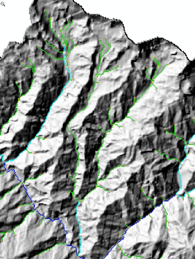 Figure 8. Stream network, with junctions in red and orange pixels
-
-
Now, find the part of the map where you want to do the chi analysis. You need to choose the junction at the downstream end of the channels where you will do your analysis. Use the identify tool (it looks like an
i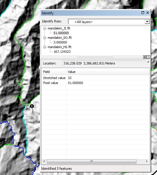 Figure 9. Finding the junction number
 -
Each junction has one and only one receiver junction, whereas it can have multiple donor junctions. When you choose a junction, the extracted channel traces down to the node one before the receiver junction. It then traces up the channel network, following the path that leads to the node the furthest flow distance from the outlet junction. That is, when junctions are reached as the algorithm moves upstream the upstream channel is determined by flow distance not drainage area. Below we show an image of this.
Extracting the .chan file
-
Now that you have the junction number, you need to run the second program. Before you run this program, you need to write a file that contains the parameters for the chi analysis.
-
The first 3 lines of this file MUST be the same as the driver file in step 1. The code does not check this so you need to make sure on your own this is the case.
-
The next two rows of the driver file are the junction number from which you want to extract the network. and something that controls how the channel network is "pruned". This is the ratio in area between the main stem and a tributary that must be exceeded for a tributary to be included in the analysis. If this number is 1 you only get the main stem. The smaller the number the more tributaries you get. A reasonable number seems to be
~0.02. Here is an example file:Mandakini 0.0001 300 76 0.01 -
There can be more information in the driver file (for example, parameters for a chi analysis), but the channel network extraction program will ignore these; it only looks at the first 5 lines of the driver function.
-
From here you run the program
chi2_write_channel_file.exe. You need to include the path name and the name of the chi parameter file. In Linux the program should be proceeded with./. Here is an example:./chi2_write_channel_file.exe /LSDTopoTools/Topographic_projects/Test_data Example_Mudd2014.driver -
This will generate several files. Note that for
fltandbilformats each dataset will consist of abiland ahdrfile.Table 19. Files generated by chi2_write_channel_file.exe. File name contains Description basinImmediately before the
.fltextension the junction number will also be listed. This file is a raster containing the outline of the contributing pixels to the basin drained by the extracted channel network.ChanNet, with extensionchanA hillshade raster. After
ChanNetthe basin number will be printed. This file is used by subsequent chi analysis: that is, further analysis does not involve the DEM, all of the necessary information is translated into the.chanfile..csv This file can be imported into ArcMap or other GIS software.
This file contain data on the nodes making up the channels in the
chanfile, but the csv file can be imported into ArcMap or QGIS. -
ArcMap should be able to see the '.csv' file.
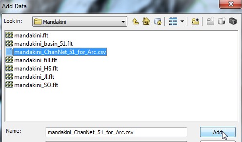 Figure 10. Adding a csv file in ArcMap
If you load this layer and right click on it, you should be able to load the xy data
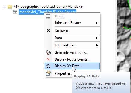 Figure 11. Showing x and y data in ArcMap
Loading the csv file will give you a shapefile with the channel nodes, and loading the
basinfile will give you the basin. Here is the basin and the channel for junction51of the Mandakini dataset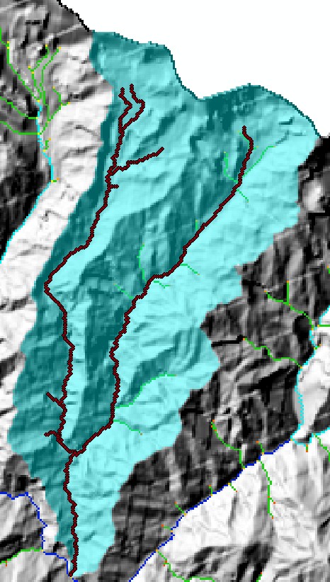 Figure 12. The extraced basin with its channels
Note how the channel extends downstream from the selected junction. It stops one node before the next junction. This way you can get an entire tributary basin that stops one node short of its confluence with the main stem channel.
Format of the .chan file
The segment fitting algorithm (see part 2) works on a "channel" file (we use the extension .chan to denote a channel file).
The channel file starts with six lines of header information that is used to reference the channel to a DEM.
f the channel is not generated from a DEM these six rows can contain placeholder values.
The six rows are:
| Keyword | Description |
|---|---|
Nrows |
number of rows |
Ncols |
number of columns |
Xllcorner |
location in the x coordinate of the lower left corner |
Yllcorner |
location in the y coordinate of the lower left corner |
Node_spacing |
the spacing of nodes in the DEM |
NoDataVal |
the value used to indicate no data |
This header information is not used in the segment analysis; it is only preserved for channel data to have some spatial reference so that scripts can be written to merge data from the channel files with DEM data.
The rest of the channel file consists of rows with 9 columns.
| Column number | paramter name | Description |
|---|---|---|
1 |
Channel number |
We use C++ style zero indexing so the main stem has channel number 0 |
2 |
Channel number of reciever channel |
The reciever channel is the channel into which this channel flows. The mainstem channel flows into itself, and currently the code can only handle simple geometries where tributaries flow into the main stem channel only, so this column is always 0. |
3 |
node number on the receiver channel |
This is the node of the reciever channel into which the tributary flows. Currently the reciever channel must be the main stem (channel 0). The main stem is defined to flow into itself. Suppose the main stem has 75 nodes. The third column would then be 74 for the main stem (because of zero indexing: the first node in the main stem channel is node 0. Nodes are organized from upstream down, so the most upstream node in the main stem channel is node zero. Suppose tributary 1 entered the main stem on the 65th node of the main stem. The third column for tributary 1 would be 64 (again, due to 0 indexing). |
4 |
node index on reciever channel |
This is the node index (generated by the LSDFlowInfo object) of the point on the reciever channel into which this channel flows. |
5 |
row |
Row in a DEM the node occupies. |
6 |
column |
Column in a DEM the node occupies. |
7 |
Flow distance (metres) |
The flow distance from the outlet of the node. It should be in metres. |
8 |
elevation (m) |
Elevation of the node. It should be in meters. |
9 |
Drainage area (m2) |
The drainage area of the node. It will be in the square of the spatial units of the DEM; if you have projected into UTM coordinates these will be in metres. |
+ Many of these columns are not used in the analysis but are there to allow the user to refer the channel file back to a DEM. Columns are separated by spaces so rows will have the format:
Chan_number receiver_chan receiver_node node_index row col flow_dist elev drainage_areaHere are the first few lines of the example file (Mandakini_ChanNet_76.chan):
648
587
290249.625
3352521.75
88.81413269
-9999
0 0 127 11457 100 223 73914.84375  4379 2382161
0 0 127 11781 101 224 73789.24219  4370 2626687.5
0 0 127 12107 102 225 73663.64062  4364.006348 2745006.75
0 0 127 12434 103 226 73538.03906  4364 2760782.5
0 0 127 12763 104 227 73412.4375  4334 2768670.5
0 0 127 12764 104 228 73323.625  4302 2910653.5
0 0 127 12765 104 229 73234.8125  4293 2989533
Now that you have the .chan file you are ready to move to the next section of the chi analysis:
part 2: constraining m/n and transforming profiles.
This may have seen like quite a few steps, but once you get familiar with the workflow the
entire process should take no more than a few minutes.
The program also prints a file in csv format that can be imported into GIS software. You will need to set the coordinate system to match that of the DEM.
11.4. Chi profile analysis, part 2: constraining m/n and transforming profiles
This is part 2 of the chi profile analysis documentation.
Part 1 can be found here in the section part 1: getting the channel profiles.
This section of the documentation assumes you have created a .chan file.
The format of the channel file is described in the section Format of the .chan file.
These "channel" files contain information about flow distance, elevation
and other properties of a channel network that are used to create a profile
transformed into so-called "chi" (\(\chi\)) space.
The transformation involves integrating drainage area along the length of the channel,
so that comparisons of channel steepness can be made for channels of different drainage area.
The analysis is similar to slope-area analysis but has some advantages; the primary advantage of the method is that it does not take the gradient of noisy topographic data, and so is less noisy than slope-area analysis.
The main disadvantage is that the method assumes channel profiles are well described by predictions of the stream power erosion law. The various advantages and disadvantages of the method are described by Perron and Royden, 2013 ESPL.
11.4.1. Steps involved to perform channel analysis
After preparing the data (see section part 1: getting the channel profiles), performing the channel analysis involves 3 steps, including visualization of the data.
11.4.2. Performing a statistical analysis to constrain the best fit m/n ratio
Once the profile data has been converted into a .chan file,
the data can then be processed to determine the most likely m/n ratio for individual channels
and also via the collinearity test (see Mudd et al (2014)).
Compiling the code
The code for running the statistical analysis to find the most likely m/n ratio can
be compiled by caling the makefile chi_m_over_n_analysis.make.
If you are using a windows machine and have installed Cygwin
you need to ensure that you have installed the make utility. However we recommend you use our vagrant setup, wherein make is installed for you.
The below instructions use the linux command prompt symbol ($),
but as long as you have make and a compiler installed on widows these
instructions should also work in a powershell terminal. See the section:
The terminal and powershells for more details.
To make the file navigate the folder that contains it and run:
$ make -f chi_m_over_n_analysis.makeThis will create the program chi_m_over_n_analysis.exe.
Running the code
The program chi_m_over_n_analysis.exe is run with 2 arguments to the command line.
-
The first argument is the path name of the path where the
.chanfile is located, along with a driver file that contains the parameters of the analysis. All data will be printed to files in this path. -
The second argument is the name of the driver file. We typically use a
.driverextension for the driver file but this is not a requirement.
For example, we call the program with:
./chi_m_over_n_analysis.exe /LSDTopoTools/Topographic_projects/Test_data Example_Mudd2014.driverThe ./ leading chi_m_over_n_analysis.exe is only necessary on a linux system.
The driver file contains a number of parameters for running the analysis.
This file is used on several different programs so not all parameters are used by chi_m_over_n_analysis.exe.
The parameters must be listed in the correct order and there cannot be any extra information between parameters
(e.g., a string describing them). The parameters are:
| Row number | Description | Notes |
|---|---|---|
1 |
The prefix of the channel file |
The original name of the DEM. If your |
2 |
Minimum slope for fill function |
Not used by |
3 |
Number of contributing pixels for a channel |
Not used by |
4 |
Junction number of channel. |
This is the junction number that was specified when the |
5 |
Area fraction for pruning |
Not used by |
6 |
\(A_0\) |
A reference drainage area for integrating to chi space (\(m^2\)). If you want to calculate channel steepness index (\(k_{sn}\)) you should set this to 1. |
7 |
Minimum segment length |
The minimum number of pixels in a segment. See Mudd et al (2014) for guidance. Values between 10-20 are recommended. The computational time required is a highly nonlinear inverse function of this parameter. 20 might lead to a run lasting a few minutes, whereas 5 might take many hours (or even days). We recommend starting with a value of 14. |
8 |
\(\sigma\) |
The standard deviation of error on the DEM, and also error from geomorphic noise (e.g., boulders in the channel). In meters. See Mudd et al (2014) paper) For SRTM this should be something like 10-30 m. The larger this number, the fewer segments you will get (see Mudd et al (2014)). |
9 |
starting \(m/n\) |
The starting \(m/n\) value to test the likelihood of. |
10 |
\(\Delta m/n\) |
The change in \(m/n\) value that you want to loop over. For example, suppose the starting \(m/n\) is 0.2 and the change in \(m/n\)is 0.05, then the next \(m/n\) value after 0.2 is 0.25. |
11 |
\(n m/n\) values |
The number of \(m/n\) values you want to loop through. |
12 |
Target nodes |
The maximum number of nodes you want to run through the partitioning algorithm at a time. Recommended values are 80-140. The computational time is nonlinearly related to this parameter, 80 might take several minutes whereas 140 will take many hours, and 200 will take months. |
13 |
Monte Carlo iterations |
The number of iterations on the Monte Carlo routine that finds the statistics for every node in the channel network rather than a subset of nodes. |
14 |
This parameters is legacy. |
Not used |
15 |
Vertical drop for \(S-A\), in meters |
The vertical drop over which slope-area analysis will be performed. |
16 |
Horizontal drop for \(S-A\), in meters |
The horizontal interval over which slope area analysis will be performed |
17 |
Max change in \(A\) (in \(m^2\)) |
The maximum change in drainage area of an interval for slope-area analysis as a fraction of the area at the midpoint of an interval. |
18 |
Target skip |
The "target skip", which is the average number of nodes the routine skips when it is trying to compute the best segments. If the DEM is 90m resolution, for example, the resolution the algorithm will work at is ~300 meters. |
And here is the cheat sheet (also included in driver_cheat_sheet.txt, which you can look at in the directory /LSDTopoTools/Git_projects/LSDTopoTools_ChiMudd2014/driver_functions_MuddChi2014/ if you used our vagrant distribution):
| Example value | Description |
|---|---|
e_bathdem |
filename prefix |
0.0001 |
minimum slope, don’t change |
300 |
N contributing pixels for a channel. Could reduce to, say 100 or even 50. |
1332 |
junction number, this will change |
0.05 |
area frac for channel pruning. 1= mainstem only, low numbers= more tribs |
1000 |
A_0 for chi analysis: probably don’t need to change. If you want to calculate channel steepness index, \(k_{sn}\), set to 1. |
20 |
minimum segment length. Should be between 5-20. |
20 |
sigma: some estimate of uncertainty in elevation data. Smaller = more segments |
0.15 |
starting m/n for best for m/n testing |
0.025 |
increment of m/n for best for m/n testing |
20 |
number of m/n values tested for m/n testing |
90 |
target length of nodes to be analy\ed for segments. Should be between 80-150 |
250 |
number of iterations for Monte Carlo analysis. 250 seems okay |
0.95 |
Not used anymore! |
20 |
Vertical interval for sampling for S-A analysis. Should be scaled to DEM resolution |
500 |
Horizontal interval for sampling for S-A analysis. Should be scaled to DEM resolution |
0.2 |
An area thinning fraction for S-A analysis. 0.2 is probably about right. |
2 |
The mean number of data nodes you skip for each node of segment analysis. For LiDAR this can be 10 or more. Nextmap can be 2-10. SRTM 0-2. |
Once this program has run, it will print out a file with the filename prefix and an extension of .movern.
| This program is computationally expensive! Increasing the target length of nodes to be analyzed and reducing the minimum segment length increases the computational time required in a highly nonlinear fashion. Increasing the skip value can reduce computational time required. |
You can expect the computation to take several minutes (e.g., minimum segment length ~20, target nodes ~100, skip set so mainstem has 300-500 nodes analysed) to many hours (e.g., minimum segment length of 5, target nodes of 120-140, skip set such that thousands of nodes are analysed).
The 'movern' file
The .movern file is produced by the statistical analysis of the channel network in order to find the most likely m/n ratio.
The filename contains information about parameter values; these are parsed by the visualisation algorithms.
The format of the filename is the filename prefix, followed by BFmovern, followed by the sigma values,
the skip value, the minimum segment length value the target nodes value and the junction number,
all separated by the underscore symbol (_). The file then has the extension .movern.
For example, the filename:
mandakini_BFmovern_20_2_20_120_51.movernIndicates that
-
\(\sigma\) = 20
-
skip = 2
-
minimum segment length = 20
-
target nodes = 120
-
and the junction number being analyzed is 51.
The format of the file is:
| Row | Value |
|---|---|
1 |
In the first column of the first row there is a placeholder value,
|
2 |
In the first column is a placeholder value,
|
3 |
In the first column is a place holder value of |
Even rows thereafter |
The first column is the channel number. The following columns are the mean \(AICc\) values for that channel. |
Odd rows thereafter |
The first column is the channel number. The following columns are the standard deviations of the \(AICc\) values for that channel. |
Here is an example file:
-99 0.15 0.175
-99 4008 4008
-99 0 0
0 2004 2004
0 0 0
1 2004 2004
1 0 0
2 2004 2004
2 0 0
3 1766.89 1788.39
3 608.033 583.88
4 1905.04 1973.54
4 422.523 238.852
5 2004 2004
5 0 0
6 1975.36 1882.18
6 224.595 450.995
Performing a sensitivity analysis on the best fit \(m/n\) ratio
For structurally or tectonically complex landscapes, it can be difficult to constrain the \(m/n\) ratio.
In such cases, it is wise to perform a sensitivity analysis of the best fit \(m/n\) ratio.
To facilitate this, we provide a python script, movern_sensitivity_driver_generation.py,
that generates a number of driver files with the parameters minimum_segment_length, sigma,
mean_skip and target_nodes that vary systematically.
To run this script you will need to change the data directory and the filename of the original driver file within the script.
You will need to modify the script before you run it. On lines 41 and 43 you need to modify the data directory and driver name of your files:
# set the directory and filename
DataDirectory =  "/LSDTopoTools/Topographic_projects/Test_data"

DriverFileName = "Example_Mudd2014.driver"
If you are running this file in Spyder from a windows machine, the path name will have slightly different formatting (you will need \\ speperators):
# set the directory and filename
DataDirectory = "c:VagrantBoxes\\LSDTopoTools\\Topographic_projects\\Test_data"| If you run from the command line you will need to navigate to the folder that contains the script. |
The script will generate driver functions with varied skip, sigma, minimum segment length and total nodes values. These will NOT be derived from the driver file you have identified, but rather will be set within the python script.
    # these are the number of different parameter values you want to use
    n_skip = 2
    n_sigma = 1
    n_msl = 2
    n_tn = 2

    # this is the starting value of the parameter values
    start_skip = 1
    start_sigma = 3.0
    start_msl = 10
    start_tn = 80

    # these are the change to the parameter value each time you iterate
    d_skip = 1
    d_sigma = 3
    d_msl = 5
    d_tn = 10
The top four variable (that start with n_) tell you how many parameter values you want to loop through,
the next four (start_) dictate where the parameter will start, and the next four (d_) dictate the change in the parameter values.
For example, if n_sigma = 3, start_sigma = 5 and d_sigma = 4, then the sigma values to be generated in .driver files will be
5, 9, and 13.
The driver files will be numbered (e.g., Example_Mudd2014.1.driver, Example_Mudd2014.2.driver, etc.):
$ ls *.driver
Example_Mudd2014.1.driver
Example_Mudd2014.2.driver
Example_Mudd2014.driver
You can run these with:
$ ./chi_m_over_n_analysis.exe /LSDTopoTools/Topographic_projects/Test_data Example_Mudd2014.1.driverOr if you want to run them with no hangup and nice:
$ nohup nice ./chi_m_over_n_analysis.exe /LSDTopoTools/Topographic_projects/Test_data Example_Mudd2014.1.driver &And then just keep running them in succession until you use up all of your CPUs (luckily at Edinburgh we have quite a few)! Sadly, this really only works if you have a cluster, so it is not so great if you are using a single Vagrant machine.
We have also written an additional python script called Run_drivers_for_mn.py which simply looks for all the drivers in folder
and sends them to your server. Once again, you’ll need to modify this python script before you run it in order to
give the script the correct data directory.
In this case the relevant line is line 18:
DataDirectory = "/LSDTopoTools/Topographic_projects/Test_data"You can run it from command line with:
$ python Run_drivers_for_mn.pyAgain, you’ll need to be in the directory holding this file to run it (but it doesn’t have to be in the same directory as the data).
| This will send all drivers to your servers to be run, so if you generated 1000 drivers, then 1000 jobs will be sent to the server. Use with caution! |
Extracting the transformed chi-elevation profiles
The next stage of the analysis is to extract the chi (\(\chi\)) profiles.
To compile the program to extract the chi profiles, you need to use the makefile chi_get_profiles.make.
The program is compiled with:
$ make -f chi_get_profiles.makeThe makefile compiles a program called chi_get_profiles.exe.
This is run, like chi_m_over_n_analysis.exe ,
with two arguments: the path name and the driver name:
$ ./chi_get_profiles.exe /LSDTopoTools/Topographic_projects/Test_data Example_Mudd2014.driverThe driver file has exactly the same format as the driver file for chi_m_over_n_analysis.exe.
A chi profile will be produced for each \(m/n\) value outlined by these elements in the driver file:
-
7th row: The starting (lowest) \(m/n\) value to test if it is the most likely.
-
8th row: The change in \(m/n\) value that you want to loop over (suppose the starting \(m/n\) is 0.2 and the change in \(m/n\) is 0.05, then the next \(m/n\) value after 0.2 is 0.25).
-
9th row: The number of \(m/n\) values you want to loop through.
Users may wish to modify these values in the driver
file from the original values to explore only
those values which have "plausible" values of the \(m/n\) ratio
(see Mudd et al (2014) for guidance).
For each \(m/n\) ratio tested, the code produces a file with the extension .tree and the string within the filename fullProfileMC_forced.
This filename also contains the \(m/n\) value so for example a filename might be called:
mandakini_fullProfileMC_forced_0.3_5_2_20_100_3124.treeThe numbers in the filename are arranged in the following order:
\(m/n\) ratio, \(\sigma\) value, mean skip, minimum segment length and target nodes.
The final number before the extension (here, 3124) is copied from the 4th row of the driver file: it is the junction number.
Users can assign different numbers to different basins to facilitate automation of data analysis.
11.4.3. The .tree file
The .tree file has as many rows as there are nodes in the channel network.
There will be more nodes in the .tree file than in the .chan file because the code extends all tributaries to the outlet.
Each row has 23 columns. The columns are
-
1st column: The channel number (like in .chan file)
-
2nd column: The receiver channel (like in .chan file)
-
3rd column: The node on receiver channel (like in .chan file)
-
4th column: The node index (like in .chan file)
-
5th column: The row of the node (like in .chan file)
-
6th column: The column of the node (like in the .chan file)
-
7th column: The flow distance of the node
-
8th column: The chi coordinate of the node
-
9th column: The elevation of the node
-
10th column: The drainage area of the node
-
11th column: The number of data points used to calculate node statistics. Because of the skipping algorithm (see Mudd et al (2013 draft manuscript)) not all nodes are analysed each iteration.
-
12th column: The mean \(M_{\chi}\) value for the node.
-
13th column: The standard deviation of the \(M_{\chi}\) value for the node.
-
14th column: The standard error of the \(M_{\chi}\) value for the node.
-
15th column: The mean \(B_{\chi}\) value for the node.
-
16th column: The standard deviation of the \(B_{\chi}\) value for the node.
-
17th column: The standard error of the \(B_{\chi}\) value for the node.
-
18th column: The mean \(DW\) value for the node.
-
19th column: The standard deviation of the \(DW\) value for the node.
-
20th column: The standard error of the \(DW\) value for the node.
-
21st column: The mean fitted elevation for the node.
-
22nd column: The standard deviation of the fitted elevation for the node.
-
23rd column: The standard error of the fitted elevation for the node.
11.4.4. Visualizing the analysis
We have also provided python scripts for visualizing the data (that is "LSDVisualisation": our code uses British spelling).
AICc_plotting.py
This script makes a plot of the \(AICc\) as a function of the \(m/n\) ratio for each channel as well as for the collinearity test. The mean and standard deviation of the \(AICc\) is plotted. In addition the \(m/n\) ratio with the minimum \(AICc\) value is highlighted, and there is a horizontal dashed line depicting the minimum \(AICc\) value plus the standard deviation of the minimum \(AICc\) value. This dashed line can help the user determine which \(m/n\) ratios are plausible (see Mudd et al (2014)). Here is an example:
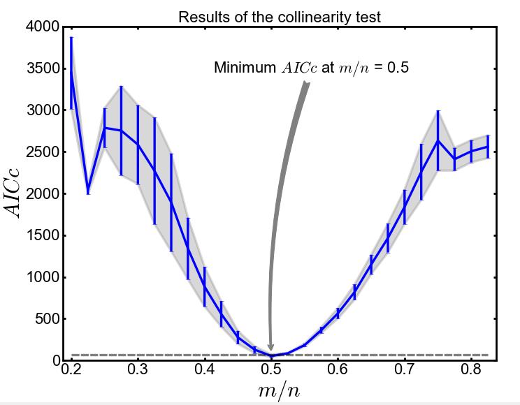
To run the AICc_plotting.py script you must modify the path name and filename after line 35 of the script.
The file it takes is a .movern file.
Plotting m/n sensitivity: AICc_plotting_multiple.py
This script looks through a directory (you need to change the DataDirectory variable in the script) for any files with BFmovern_.movern
in them and plots the \(AICc\) results.
The code extracts the parameter values from the filename so each plotted figure has the parameter values in the title.
Note that this script plots to file instead of to screen.
You can change the kind of output file by changing the parameter OutputFigureFormat.
See MatPlotLib documentation for options, but possibilities include jpg and pdf.
Plotting chi profiles and \(M_{\chi}\) values chi_visualisation.py
This script makes three figures.
First, you must define the path name and the filename after line 39 of the script.
This script takes a .tree file. The first figure is a plot of the channels in chi (\(\chi\)) space.
The transformed data is in a semi-transparent solid line and the best fit segments are in dashed lines.
Each tributary is plotted with a different colour. Here is an example:
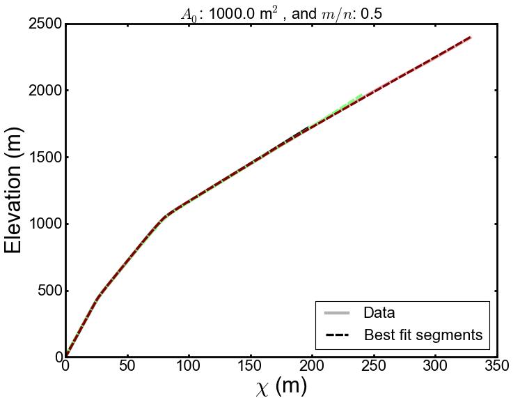
| These examples are derived from numerical model landscapes and are "perfect". Natural channels will be considerably noisier.** |
The second figure generated by this script is a figure showing the gradient in \(\chi\)-elevation space as a function of \(\chi\). The gradient in \(\chi\)-elevation is indicative of a combination of erosion rate and erodibility, so these plots allow perhaps a clearer idea of the different segments identified by the segment fitting algorithms. The colour scheme from the first figure is carried forward, so that it is easy to identify the characteristics of each tributary. Here is an example:
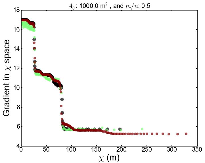
The third figure displays the longitudinal channel profiles (elevation as a function of flow distance), but these channel profiles are coloured by the gradient in \(\chi\)-elevation space. Here is an example:
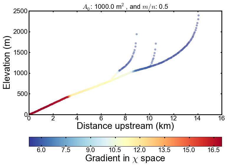
Plotting the sensitivity of best fit \(m/n\) values to parameters: bf_movern_sensitivity.py
This script looks in the directory DataDirectory for all the files with BFmovern_.movern in the filename and then compiles the best fit \(m/n\) ratio from these files. It then produces box and whisker plots of the best fit \(m/n\) ratio. The red line is the median \(m/n\) ratio, the box shows the 25th and 75th percentile \(m/n\) ratios, the whiskers show the data range, with outliers (as determined by the Matplotlib function boxplot) as "+" symbols. The boxes are notched; these give 85% confidence intervals to the median value after bootstrapping 10,000 times. Here is an example plot:
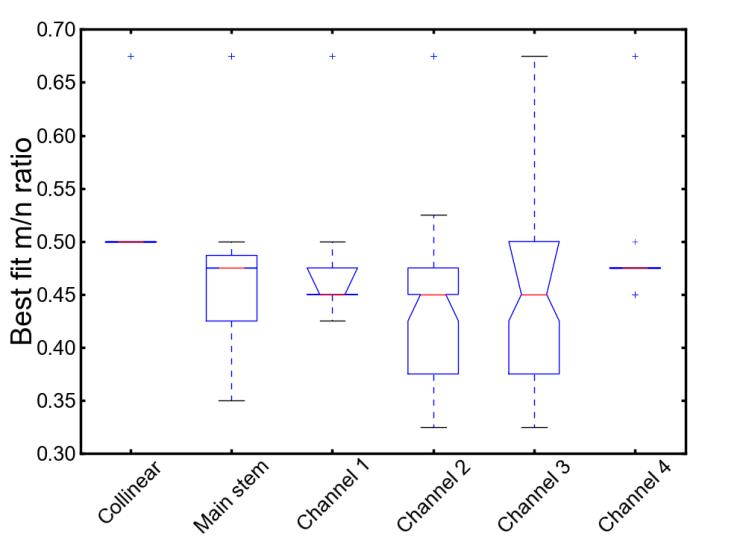
Plotting the spatial distribution of \(M_{\chi}\) values: raster_plotter_2d_only.py
This script contains two functions. One is for plotting the tributaries superimposed on a hillshade (or any other raster) and another is for plotting the \(M_{\chi}\) values superimposed on a raster (we usually do this on the hillshade).
For this to work, the .chan file must be referenced to a coordinate system.
That means that the row and column information in the .chan file corresponds to the xllcorner, yllcorner and
node spacing data in the first few lines of the .chan file.
If you have the LSDTopoToolbox this will happen automatically, but if you are writing a script to generate your own
.chan files you`ll need to ensure that your channel nodes have the correct row and column data.
The DEM used for the hillshade does not need to be the same as the DEM used for the .chan file
(that is, it can have different n_rows and n_columns etc, so you can, in principle,
do a chi analysis on a clipped version of a DEM but then plot the results on the full DEM extent).
The two functions are:
-
coloured_chans_like_graphs: This takes two strings: the filename of the raster and the filename of the.treefile. You have to include the full path name for both of these files.The colouring scheme used for the channels is the same as in the
elevationand \(M_{\chi}\) plots made bychi_visualisation.py. Here is an example: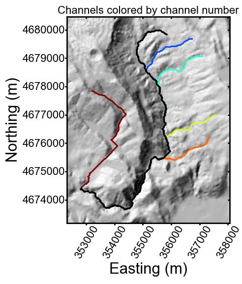 Figure 18. A map showing the channels (colored by their number) within a basin
 -
m_values_over_hillshade: Again, this takes two strings: the filename of the raster and the filename of the.treefile. You have to include the full path name for both of these files.The colouring scheme on the \(M_{\chi}\) values is the same as in the
chi_visualisation.pyplot where \(M_{\chi}\) is plotted on the channel profile. Here is an example: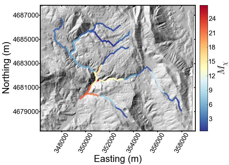 Figure 19. The \(M_{\chi}\) of channels within a basin
To run one or the other of these function you need to scroll to the bottom of the script and comment or uncomment one of the function lines.
11.4.5. A Sample Chi Analysis Workflow
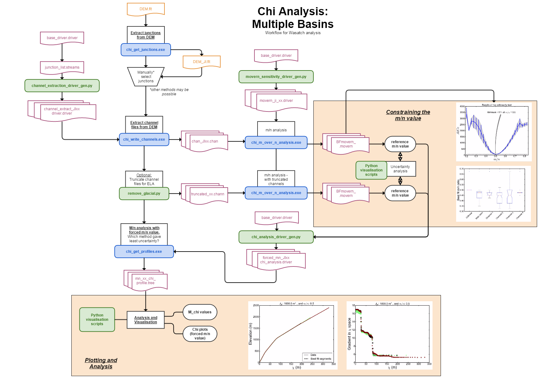
11.5. Chi analysis part 3: Getting chi gradients for the entire landscape
The algorithms in the previous two sections were designed for users to statistically determine the \(m/n\) ratio of a given landscape. The routines calculate the gradient in chi space (which we call \(M_{\chi}\)) but they focus on the main stem (which in our code is calculated with the longest channel) and its biggest tributaries.
In many applications, however, users may with to map the chi gradient across a landscape. We provide a tool for doing so in the driver function 'map_chi_gradient.cpp'.
11.5.1. Compile the code
The chi gradient mapping tool can be compiled by navigating to the driver function folder and running make. If you are using our vagrant setup you can go directly to the correct folder by typing cd /LSDTopoTools/Git_projects/LSDTopoTools_ChiMudd2014/driver_functions_MuddChi2014/. Once there, run the command:
$ make -f chi_mapping_tool.make11.5.2. Run the map chi gradient tool
The program is now ready to run with the correct inputs. The function takes two inputs
-
The path to the parameter file. This MUST inclde the trailing slash (i.e.,
/LSDTopoTools/Topographic_projects/Test_datais incorrect whereas/LSDTopoTools/Topographic_projects/Test_data/is correct). -
The name of the parameter file.
So if the parameter file is located at /LSDTopoTools/Topographic_projects/Test_data and it is called test_chi_map.param, you run the program with:
$ ./chi_mapping_tool.exe /LSDTopoTools/Topographic_projects/Test_data test_chi_map.paramAs we will see momentarily, the data an the parameter file can be in different locations, although in general it might be sensible to place the parameter file in the sample directory as the data.
The code is run using a parameter file, within which users can set the data they want to print to file. Regardless of which data they choose to print to file, a file will be printed with the extension _Input.param which prints out all the parameters used in the analysis (including the default parameters). This file can be used to verify if the correct parameters have been used in the analysis.
11.5.3. The parameter file
The parameter file has keywords followed by a value. The format of this file is similar to the files used in the LSDTT_analysis_from_paramfile program, which you can read about in the section Running your first analysis.
The parameter file has a specific format, but the filename can be anything you want. We tend to use the extensions .param and .driver for these files, but you could use the extension .MyDogSpot if that tickled your fancy.
|
The parameter file has keywords followed by the : character. After that there is a space and the value.
11.5.4. Parameter file options
Below are options for the parameter files. Note that all DEMs must be in ENVI bil format (DO NOT use ArcMap’s bil format: these are two different things. See the section What data does LSDTopoToolbox take? if you want more details).
The reason we use bil format is because it retains georeferencing which is essential to our file output since many of the files output to csv format with latitude and longitude as coordinates.
| Keyword | Input type | Description |
|---|---|---|
write path |
string |
The path to which data is written. The code will NOT create a path: you need to make the write path before you start running the program. |
read path |
string |
The path from which data is read. |
write fname |
string |
The prefix of rasters to be written without extension.
For example if this is |
read fname |
string |
The filename of the raster to be read without extension. For example if the raster is |
channel heads fname |
string |
The filename of a channel heads file. You can import channel heads. If this is set to |
| Keyword | Input type | Default value | Description |
|---|---|---|---|
min_slope_for_fill |
float |
0.001 |
The minimum slope between pixels for use in the fill function. |
threshold_contributing_pixels |
int |
1000 |
The number of pixes required to generate a channel (i.e., the source threshold). |
minimum_basin_size_pixels |
int |
1000 |
The minimum number of pixels in a basin for it to be retained. This operation works on the baselevel basins: subbasins within a large basin are retained. |
test_drainage_boundaries |
bool (true or 1 will work) |
false |
A boolean that, if set to true, will eliminate basins with pixels drainage from the edge. This is to get rid of basins that may be truncated in a DEM (and thus will have incorrect chi values). |
only_take_largest_basin |
bool (true or 1 will work) |
true |
If this is true, a chi map is created based only upon the largest basin in the raster. |
| Keyword | Input type | Default value | Description |
|---|---|---|---|
A_0 |
float |
1000 |
The A0 parameter (which nondimensionalises area) for chi analysis. This is in m2. |
m_over_n |
float |
0.5 |
The m/n paramater (sometimes known as the concavity index) for calculating chi. |
threshold_pixels_for_chi |
int |
1000 |
The number of contributing pixels above which chi will be calculated. The reason for the threshold is to produce chi plots that do not extend onto hillslopes; this helps visualisation of chi differences between nearby headwater channels. |
| Keyword | Input type | Default value | Description |
|---|---|---|---|
n_iterations |
int |
20 |
The number of iterterations of random sampling of the data to construct segments. The sampling probability of individual nodes is determined by the skip parameter. |
target_nodes |
int |
80 |
The number of nodes in a segment finding routine. Channels are broken into subdomains of aroung this length and then segmenting occurs on these subdomains. |
minimum_segment_length |
int |
10 |
The minimum length of a segment in sampled data nodes. The actual length is approxamately this parameter times (1+skip). |
skip |
int |
2 |
During Monte Carlo sampling of the channel network, nodes are sampled by skipping nodes after a sampled node. The skip value is the mean number of skipped nodes after each sampled node. For example, if skip = 1, on average every other node will be sampled. Skip of 0 means every node is sampled (in which case the n_iterations should be set to 1, because there will be no variation in the fit between iterations). |
sigma |
float |
10.0 |
This represents the variability in elevation data (if the DEM has elevation in metres, then this parameter will be in metres). It should include both uncertainty in the elevation data as well as the geomorphic variability: the size of roughness elements, steps, boulders etc in the channel that may lead to a channel profile diverging from a smooth long profile. |
basic_Mchi_regression_nodes |
int |
11 |
This works with the basic chi map: segments are not calculated. Instead, a moving window, with a length set by this parameter, is moved over the channel nodes to calculate the chi slope. This method is very similar to methods used to calculate normalised channel steepness (ksn). |
| Input type | Description |
|---|---|
only_check_parameters |
If this is true, the program simply prints all the parameters to a file and does not perform any analyses. This is used for checking if the parameters are set correctly and that the keywords are correct. |
print_stream_order_raster |
If true, prints a raster of the stream orders. |
print_junction_index_raster |
If true, prints a raster with the junction indices. |
print_fill_raster |
If true, prints a filled raster |
print DrainageArea_raster |
If true, prints a raster of the draiange area in m2. |
print_chi_coordinate_raster |
If true, prints a raster with the chi coordinate (in m). Note that if you want to control the size of the data symbols in a visualisation, you should select the |
print_simple_chi_map_to_csv |
If true, prints a csv file with latitude, longitude and the chi coordinate. Can be converted to a shapefile or GeoJSON with our python mapping scripts. This options gives more flexibility in visualisation than the raster, since in the raster data points will only render as one pixel. |
print_segmented_M_chi_map_to_csv |
If true, prints a csv file with latitude, longitude and a host of chi information including the chi slope, chi intercept, drainage area, chi coordinate and other features of the drainage network. The \(M_{\chi}\) values are calculated with the segmentation algorithm of Mudd et al. 2014. |
print_basic_M_chi_map_to_csv |
If true, prints a csv file with latitude, longitude and a host of chi information including the chi slope, chi intercept, drainage area, chi coordinate and other features of the drainage network. The \(M_{\chi}\) values are calculated with a rudimentary smoothing window that has a size determined by the parameter |
11.5.5. Example parameter file
Below is an exaple parameter file. This file is included in the repository along with the driver functions.
# Parameters for performing chi analysis
# Comments are preceeded by the hash symbol
# Documentation can be found here:
# http://lsdtopotools.github.io/LSDTT_book/#_chi_analysis_part_3_getting_chi_gradients_for_the_entire_landscape

# These are parameters for the file i/o
# IMPORTANT: You MUST make the write directory: the code will not work if it doens't exist.
read path: /LSDTopoTools/Topographic_projects/Test_data
write path: /LSDTopoTools/Topographic_projects/Test_data
read fname: Mandakini
channel heads fname: NULL

# Parameter for filling the DEM
min_slope_for_fill: 0.0001

# Parameters for selecting channels and basins

threshold_contributing_pixels: 200000
minimum_basin_size_pixels: 50000
test_drainage_boundaries: false

# Parameters for chi analysis
A_0: 1000
m_over_n: 0.45
threshold_pixels_for_chi: 20000

n_iterations: 20
target_nodes: 80
minimum_segment_length: 10
sigma: 10.0
skip: 2

# The data that you want printed to file
only_check_parameters: true
print_stream_order_raster: false
print_DrainageArea_raster: false
print_segmented_M_chi_map_to_csv: true
11.5.6. Output data formats
Data is written to either rasters or csv files. The rasters are all in bil format, which you can read about in the section: What data does LSDTopoToolbox take?
The csv files are comma seperated value files which can be read by spreadsheets and GIS software. These files all have labeled columns so their contents can be easily views. All of the files contain latitude and longitude columns. These columns are projected into the WGS84 coordinate system for ease of plotting in GIS software.
Viewing data and converting to GIS ready formats
If the user has opted to print data in csv format, they can use our visualisation tools to convert the data into GIS-ready formats.
Users should first clone the mapping tools respoitory:
$ git clone https://github.com/LSDtopotools/LSDMappingTools.gitIn this repository the user needs to get a helping script called LSDOSystemTools.py. You can fetch this script using the wget tool:
$ wget https://github.com/LSDtopotools/LSDAutomation/raw/master/LSDOSystemTools.pyThe user can then run the script TestMappingToolsPoint.py, activating the TestMappingToolsLassoCSV function:
if __name__ == "__main__":
    TestMappingToolsLassoCSV()
and changing the target directory to the directory storing the csv files:
def TestMappingToolsLassoCSV():
    DataDirectory = "C://VagrantBoxes//LSDTopoTools//Topographic_projects//Test_data//"
    LSDP.ConvertAllCSVToGeoJSON(DataDirectory)
Note that this is if your run the python script within windows. If you run it within your agrant Linux machine the directory would be:
def TestMappingToolsLassoCSV():
    DataDirectory = "/LSDTopoTools/Topographic_projects/Test_data/"
    LSDP.ConvertAllCSVToGeoJSON(DataDirectory)
You can convert all csv files into either shapefiles or GeoJSON files.
    LSDP.ConvertAllCSVToGeoJSON(DataDirectory)
    LSDP.ConvertAllCSVToShapefile(DataDirectory)
These files can then be read by your favourite GIS.
11.6. Summary
You should now be able to extract some simple topographic metrics from a DEM using our Driver_analysis program.
12. Basin averaged cosmogenic analysis
We have developed a toolkit to automate calculation of basin (or catchement) averaged denudation rates estimated from the concentration of in situ cosmogenic nuclides in stream sediment. This toolkit is called the CAIRN method. Currently 10Be and 26Al are supported.
If you use this to calculate denudation rates that are later published, please cite this paper:
Mudd, S. M., Harel, M.-A., Hurst, M. D., Grieve, S. W. D., and Marrero, S. M.: The CAIRN method: automated, reproducible calculation of catchment-averaged denudation rates from cosmogenic nuclide concentrations, Earth Surf. Dynam., 4, 655-674, doi:10.5194/esurf-4-655-2016, 2016.
The toolkit requires:
-
Data on cosmogenic samples.
-
A file containing filenames of the topographic data, and optional filenames for shielding rasters.
-
A parameter file.
The toolkit then produces:
-
A csv file that contains results of the analysis.
-
A text file that can be copied into the CRONUS online calculator for data comparison.
12.1. Get the code and data basin-averaged cosmogenic analysis
This section goes walks you through getting the code and example data, and also describes the different files you will need for the analysis.
12.1.1. Get the source code for basin-averaged cosmogenics
First navigate to the folder where you will keep your repositories.
In this example, that folder is called /home/LSDTT_repositories.
In a terminal window, go there with the cd command:
$ cd /home/LSDTT_repositories/You can use the pwd command to make sure you are in the correct directory.
If you don’t have the directory, use mkdir to make it.
Clone the code from Git
Now, clone the repository from GitHub:
$ pwd
/home/LSDTT_repositories/
$ git clone https://github.com/LSDtopotools/LSDTopoTools_CRNBasinwide.git
Alternatively, get the zipped code
If you don’t want to use git, you can download a zipped version of the code:
$ pwd
/home/LSDTT_repositories/
$ wget https://github.com/LSDtopotools/LSDTopoTools_CRNBasinwide/archive/master.zip
$ gunzip master.zip
GitHub zips all repositories into a file called master.zip,
so if you previously downloaded a zipper repository this will overwrite it.
|
Compile the code
Okay, now you should have the code. You will still be sitting in the directory
/home/LSDTT_repositories/, so navigate up to the directory LSDTopoTools_BasinwideCRN/driver_functions_BasinwideCRN/.
$ pwd
/home/LSDTT_repositories/
$ cd LSDTopoTools_CRNBasinwide
$ cd driver_functions_CRNBasinwide
There are a number of makefiles (thse with extension .make in this folder).
These do a number of different things that will be explained later in this chapter.
12.1.2. Getting example data: The San Bernardino Mountains
We have provided some example data. This is on our Github example data website.
The example data has a number of digital elevation models in various formats, but for these examples we will be only using one dataset, from the San Bernardino Mountains in California.
You should make a folder for your data using mkdir somewhere sensible.
For the purposes of this tutorial I’ll put it in the following folder:
$ pwd
/home/ExampleDatasets/SanBernardino/
Again, we will only take the data we need, so use wget to download the data:
$ wget https://github.com/LSDtopotools/ExampleTopoDatasets/raw/master/SanBern.bil
$ wget https://github.com/LSDtopotools/ExampleTopoDatasets/raw/master/SanBern.hdr
$ wget https://github.com/LSDtopotools/ExampleTopoDatasets/raw/master/example_parameter_files/SanBern_CRNData.csv
$ wget https://github.com/LSDtopotools/ExampleTopoDatasets/raw/master/example_parameter_files/SanBern_CRNRasters.csv
$ wget https://github.com/LSDtopotools/ExampleTopoDatasets/raw/master/example_parameter_files/SanBern.CRNParam
You should now have the following files in your data folder:
$ pwd
/home/ExampleDatasets/SanBernardino/
$ ls
SanBern.bil    SanBern_CRNData.csv     SanBern.CRNParam
SanBern.hdr    SanBern_CRNRasters.csv
The file SanBern_CRNRasters.csv will need to be modified with the appropriate paths to your files! We will describe how to do that below.
|
12.1.3. Setting up your data directories and parameter files
Before you can run the code, you need to set up some data structures.
| If you downloaded the example data, these files will already exist. These instructions are for when you need to run CRN analysis on your own datasets. |
-
You can keep your topographic data separate from your cosmogenic data, if you so desire. You’ll need to know the directory paths to these data.
-
In a single folder (again, it can be separate from topographic data), you must put a i) parameter file, a cosmogenic data file, and a raster filenames file .
-
These three files must have the same prefix, and each have their own extensions.
-
The parameter file has the extension:
.CRNParam. -
The cosmogenic data file has the extension
_CRNData.csv. -
The raster filenames file has the extension
_CRNRasters.csv.
-
-
For example, if the prefix of your files is
SanBern, then your three data files will beSanBern.CRNParam,SanBern_CRNData.csv, andSanBern_CRNRasters.csv. -
If the files do not have these naming conventions, the code WILL NOT WORK! Make sure you have named your files properly.
The parameter file
The parameter file contains some values that are used in the calculation of both shielding and erosion rates.
This file must have the extension .CRNParam. The extension is case sensitive.
|
The parameter file could be empty, in which case parameters will just take default values. However, you may set various parameters. The format of the file is:
parameter_name: parameter_valueSo for example a parameter file might look like:
min_slope: 0.0001
source_threshold: 12
search_radius_nodes: 1
threshold_stream_order: 1
theta_step: 30
phi_step: 30
Muon_scaling: Braucher
write_toposhield_raster: true
write_basin_index_raster: true
There cannot be a space between the parameter name and the ":" character,
so min_slope : 0.0002 will fail and you will get the default value.
|
In fact all of the available parameters are listed above, and those listed above are default values. The parameter names are not case sensitive. The parameter values are case sensitive. These parameters are as follows:
| Keyword | Input type | default | Description |
|---|---|---|---|
min_slope |
float |
0.0001 |
The minimum slope between pixels used in the filling function (dimensionless) |
source_threshold |
int |
12 |
The number of pixels that must drain into a pixel to form a channel. This parameter makes little difference, as the channel network only plays a role in setting channel pixels to which cosmo samples will snap. This merely needs to be set to a low enough value that ensures there are channels associated with each cosmogenic sample. |
search_radius_nodes |
int |
1 |
The number of pixels around the location of the cosmo location to search for a channel. The appropriate setting will depend on the difference between the accuracy of the GPS used to collect sample locations and the resolution of the DEM. If you are using a 30 or 90m DEM, 1 pixel should be sufficient. More should be used for LiDAR data. |
threshold_stream_order |
int |
1 |
The minimum stream or which the sample snapping routine considers a 'true' channel. The input is a Strahler stream order. |
theta_step |
int |
30 |
Using in toposhielding calculations. This is the step of azimuth (in degrees) over which shielding and shadowing calculations are performed. Codilean (2005) recommends 5, but it seems to work without big changes differences with 15. An integer that must be divisible by 360 (although if not the code will force it to the closest appropriate integer). |
phi_step |
int |
30 |
Using in toposhielding calculations. This is the step of inclination (in degrees) over which shielding and shadowing calculations are performed. Codilean (2005) recommends 5, but it seems to work without big changes differences with 10. An integer that must be divisible by 360 (although if not the code will force it to the closest appropriate integer). |
path_to_atmospheric_data |
string |
./ |
The path to the atmospheric data. DO NOT CHANGE. This is included in the repository so should work if you have cloned our git repository. Moving this data and playing with the location the atmospheric data is likeley to break the program. |
Muon_scaling |
string |
Braucher |
The scaling scheme for muons. Options are "Braucher", "Schaller" and "Granger". If you give the parameter file something other than this it will default to Braucher scaling. These scalings take values reported in COSMOCALC as described by Vermeesch 2007. |
write_toposhield_raster |
bool |
true |
If true this writes a toposhielding raster if one does not exist. Saves a bit of time but will take up some space on your hard disk! |
write_basin_index_raster |
bool |
true |
For each DEM this writes an LSDIndexRaster to file with the extension |
write_full_scaling_rasters |
bool |
true |
This writes three rasters if true: a raster with |
The cosmogenic data file
This file contains the actual cosmogenic data: it has the locations of samples, their concentrations of cosmogenics (10Be and 26Al) and the uncertainty of these concentrations.
The cosmogenic data file must have the extension _CRNData.csv.
The extension is case sensitive.
|
This is a .csv file: that is a comma separated value file. It is in that format to be both excel and
pandas friendly.
The first row is a header that names the columns, after that there should be 7 columns (separated by commas) and unlimited rows. The seven columns are:
sample_name, sample_latitude, sample_longitude, nuclide, concentration, AMS_uncertainty, standardisation
An example file would look like this (this is not real data):
Sample_name,Latitude,Longitude,Nuclide,Concentration,Uncertainty,Standardisation
LC07_01,-32.986389,-71.4225,Be10,100000,2500,07KNSTD
LC07_04,-32.983528,-71.415556,Be10,150000,2300,07KNSTD
LC07_06,-32.983028,-71.415833,Al26,4000,2100,KNSTD
LC07_08,-32.941333,-71.426583,Be10,30000,1500,07KNSTD
LC07_10,-33.010139,-71.435389,Be10,140000,25000,07KNSTD
LC07_11,-31.122417,-71.576194,Be10,120502,2500,07KNSTD
Or, with reported snow shielding:
Sample_name,Latitude,Longitude,Nuclide,Concentration,Uncertainty,Standardisation, Snow_shielding
LC07_01,-32.986389,-71.4225,Be10,100000,2500,07KNSTD,0.7
LC07_04,-32.983528,-71.415556,Be10,150000,2300,07KNSTD,0.8
LC07_06,-32.983028,-71.415833,Al26,4000,2100,KNSTD,1.0
LC07_08,-32.941333,-71.426583,Be10,30000,1500,07KNSTD,1.0
LC07_10,-33.010139,-71.435389,Be10,140000,25000,07KNSTD,1.0
LC07_11,-31.122417,-71.576194,Be10,120502,2500,07KNSTD,0.987
If you followed the instructions earlier in the section Getting example data: The San Bernardino Mountains
then you will have a CRNdata.csv file called Binnie_CRNData.csv in your data folder.
| Column | Heading | type | Description |
|---|---|---|---|
1 |
Sample_name |
string |
The sample name NO spaces or underscore characters! |
2 |
Latitude |
float |
Latitude in decimal degrees. |
3 |
Longitude |
float |
Longitude in decimal degrees. |
4 |
Nuclide |
string |
The nuclide. Options are |
5 |
Concentration |
float |
Concentration of the nuclide in atoms g-1. |
6 |
Uncertainty |
float |
Uncertainty of the concentration of the nuclide in atoms g-1. |
7 |
Standardization |
float |
The standardization for the AMS measurments. See table below for options. |
8 |
Reported snow shielding |
float |
The reported snow shielding value for a basin. Should be a ratio between 0 (fully shielded) and 1 (no shielding). This column is OPTIONAL. |
| Nuclide | Options |
|---|---|
10Be |
|
26Al |
|
The raster names file
This file contains names of rasters that you want to analyze.
The raster names file must have the extension _CRNRasters.csv.
The extension is case sensitive.
|
This file is a csv file that has as many rows as you have rasters that cover your CRN data. Each row can contain between 1 and 4 columns.
-
The first column is the FULL path name to the Elevation raster and its prefix (that is, without the
.bil, e.g.:/home/smudd/basin_data/Chile/CRN_basins/Site01/Site_lat26p0_UTM19_DEM -
The next column is either a full path name to a snow shielding raster or a snow shielding effective depth. Both the raster and the single value should have units of g/cm^2 snow depth. If there is no number here the default is 0.
-
The next column is either a full path name to a self shielding raster or a self shielding effective depth. Both the raster and the single value should have units of g/cm2 shielding depth. If there is no number here the default is 0.
-
The next column is the FULL path to a toposhielding raster. If this is blank the code will run topographic shielding for you.
topographic shielding is the most computationally demanding step in the cosmo analysis. A typical file might will look like this:
An example CRNRasters.csv file/home//basin_data/Site01/Site01_DEM,0,0,/home/basin_data/Site01/Site01_DEM_TopoShield /home/basin_data/Site02/Site02_DEM,5,10 /home/basin_data/Site03/Site03_DEM,5,/home/basin_data/Site03/Site03_DEM_SelfShield /home/basin_data/Site04/Site04_DEM,/home/basin_data/Site04/Site04_DEM_SnowShield,/home/basin_data/Site04/Site04_DEM_SelfShield /home/basin_data/Site05/Site05_DEM /home/basin_data/Site06/Site06_DEM,/home/basin_data/Site06/Site06_DEM_SnowShield
| Column | Heading | type | Description |
|---|---|---|---|
1 |
Path and prefix of elevation data |
string |
Path and prefix of elevation data; does not include the extension (that is, does not include |
2 |
Snow shielding |
float or string or empty |
This could be empty, or contain a float, in which case it is the effective depth of snow (g cm-2) across the entire basin or a string with the path and file prefix of the snow depth (g cm-2) raster. If empty, snow depth is assumed to be 0. |
3 |
Self shielding |
float or string or empty |
This could be empty, or contain a float, in which case it is the effective depth of material eroded(g cm-2) across the entire basin or a string with the path and file prefix of the eroded depth (g cm-2) raster. If empty, eroded depth is assumed to be 0. |
4 |
Topo shielding |
string or empty |
This could be empty or could contain a string with the path and file prefix of the topographic shielding (a ratio between 0 and 1) raster. If empty topographic shielding is assumed to be 1 (i.e., no shielding). |
12.1.4. Modifying your CRNRasters file the python way
The _CRNRasters.csv file contains the path names and the file prefixes of the rasters to be used in the analysis.
The paths will vary depending on your own file structures.
Updating these paths by hand can be quite tedious, so we have prepared a python script to automate this process.
You can get this script here:
$ wget https://github.com/LSDtopotools/LSDAutomation/raw/master/LSDOSystemTools.py
$ wget https://github.com/LSDtopotools/LSDAutomation/raw/master/PrepareCRNRastersFileFromDirectory.pyThe script LSDOSystemTools.py contians some tools for managing paths and files, the actual work is done by the script PrepareCRNRastersFileFromDirectory.py.
In an editor, go into PrepareCRNRastersFileFromDirectory.py and navigate to the bottom of the file.
Change the path to point to the directory with your DEMs. The prefix is the prefix of your files, so in this example change prefix to SanBern.
You can then run the script with:
$ python PrepareCRNRastersFileFromDirectory.pyThis script will then update the _CRNRasters.csv file to reflect your directory structure. The script also detects any associated shielding rasters.
12.2. Calculating Topographic Shielding
Cosmogenic nuclides are produced at or near the Earth’s surface by cosmic rays, and these rays can be blocked by topography (i.e., big mountains cast "shadows" for cosmic rays).
In most cases, you will not have topographic shielding rasters available, and will need to calculate these.
Shielding calculation are computationally intensive, much more so than the actual erosion rate computations. Because of the computational expense of shielding calculations, we have prepared a series of tools for speeding this computation.
The topographic shielding routines take the rasters from the _CRNRasters.csv file and the _CRNData.csv file and computes the location of all CRN basins.
They then clips a DEM around the basins (with a pixel buffer set by the user).
These clipped basins are then used to make the shielding calculations and the erosion rate calculations.
This process of clipping out each basin spans a large number of new DEM that require a new directory structure. A python script is provided to set up this directory structure in order to organize the new rasters.
| This process uses a large amount of storage on the hard disk because a new DEM will be written for each CRN basin. |
12.2.1. Steps for preparing the rasters for shielding calculations
Creation of subfolders for your topographic datasets
The first step is to create some subfolders to store topographic data. We do this using a python script
-
First, place the
_CRNRasters.csvand_CRNData.csvfile into the same folder, and make sure the_CRNRasters.csvfile points to the directories that contain the topographic data. If you are working with the example data (see section Getting example data: The San Bernardino Mountains), you should navigate to the folder with the data (for this example, the folder is in/home/ExampleDatasets/SanBernardino/):$ pwd /home/ExampleDatasets/SanBernardino/ $ ls SanBern_CRNData.csv SanBern_CRNRasters.csv SanBern.hdr SanBern.bil SanBern.CRNparamYou will then need to modify
SanBern_CRNRasters.csvto reflect your directory:Modify yourSanBern_CRNRasters.csvfile/home/ExampleDatasets/SanBernardino/SanBernEach line in this file points to a directory holding the rasters to be analyzed.
In this case we are not supplying and shielding rasters. For more details about the format of this file see the section: The raster names file.
-
Second, run the python script
PrepareDirectoriesForBasinSpawn.py.-
You can clone this script from GitHub; find it here: https://github.com/LSDtopotools/LSDAutomation You will also need the file
LSDOSystemTools.pyfrom this repository. TheLSDOSystemTools.pyfile contains some scripts for making sure directories are in the correct format, and for changing filenames if you happen to be switching between Linux and Windows. It is unlikely that you will need to concern yourself with its contents, as long as it is present in the same folder as thePrepareDirectoriesForBasinSpawn.pyfile.The scripts can be downloaded directly using:
$ wget https://github.com/LSDtopotools/LSDAutomation/raw/master/PrepareDirectoriesForBasinSpawn.py $ wget https://github.com/LSDtopotools/LSDAutomation/raw/master/LSDOSystemTools.py -
You will need to scroll to the bottom of the script and change the
path(which is simply the directory path of the_CRNRasters.csvfile. -
You will need to scroll to the bottom of the script and change the
prefix(which is simply prefix of the_CRNRasters.csvfile; that is the filename before_CRNRasters.csvso if the filename isYoYoMa_CRNRasters.csvthenprefixisYoYoMa. Note this is case sensitive.In this example, scroll to the bottom of the file and change it to:
if __name__ == "__main__": path = "/home/ExampleDatasets/SanBernardino" prefix = "SanBern" PrepareDirectoriesForBasinSpawn(path,prefix) -
This python script does several subtle things like checking directory paths and then makes a new folder for each DEM. The folders will contain all the CRN basins located on the source DEM.
If you are using the example data, the rather trivial result will be a directory called
SanBern.
-
Spawning the basins
Now you will run a C++ program that spawns small rasters that will be used for shielding calculations. First you have to compile this program.
-
To compile, navigate to the folder
/home/LSDTT_repositories/LSDTopoTools_CRNBasinwide/driver_functions_CRNBasinwide/. If you put the code somewhere else, navigate to that folder. Once you are in the folder with the driver functions, type:$ make -f Spawn_DEMs_for_CRN.make -
The program will then compile (you may get some warnings—ignore them.)
-
In the
/driver_functions_CRNTools/folder, you will now have a programSpawn_DEMs_for_CRN.exe. You need to give this program two arguments. -
You need to give
Spawn_DEMs_for_CRN.exe, the path to the data files (i.e.,_CRNRasters.csvand_CRNData.csv), and the prefix, so if they are calledYoMa_CRNRaster.csvthe prefix isYoMa). In this example the prefix will beSanBern. Run this with:PS> Spawn_DEMs_for_CRN.exe PATHNAME DATAPREFIXin windows or:
$ ./Spawn_DEMs_for_CRN.exe PATHNAME DATAPREFIXin Linux.
In our example, you should run:
$ ./Spawn_DEMs_for_CRN.exe /home/ExampleDatasets/SanBernardino/ SanBernThe PATHNAME MUST have a frontslash at the end. /home/ExampleDatasets/SanBernardino/will work whereas/home/ExampleDatasets/SanBernardinowill lead to an error. -
Once this program has run, you should have subfolders containing small DEMs that contain the basins to be analyzed. There will be one for every cosmogenic sample that lies within the DEM.
-
You will also have files that contain the same
PATHNAMEandPREFIXbut have_Spawnedadded to the prefix. For example, if your original prefix wasCRN_test, the new prefix will beCRN_test_Spawned. -
In the file
PREFIX_Spawned_CRNRasters.csvyou will find the paths and prefixes of all the spawned basins.
12.2.2. The shielding computation
The shielding computation is the most computationally expensive step of the CRN data analysis. Once you have spawned the basins (see above section, Steps for preparing the rasters for shielding calculations), you will need to run the shielding calculations.
-
You will first need to compile the program that calculates shielding. This can be compiled with:
$ make -f Shielding_for_CRN.make -
The compiled program (
Shielding_for_CRN.exe) takes two arguments: thePATHNAMEand thePREFIX. -
You could simply run this on a single CPU after spawning the basins; for example if the original data had the prefix
CRN_testbefore spawning, you could run the program with:$ ./Shielding_for_CRN.exe PATHNAME CRN_test_Spawnedwhere
PATHNAMEis the path to your_CRNRasters.csv,_CRNData.csv, and.CRNParam(these files need to be in the same path).If you only wanted to do a subset of the basins, you can just delete rows from the *_Spawned_CRNRasters.csvfile as needed.
This will produce a large number of topographic shielding rasters (with _SH in the filename), for example:
smudd@burn SanBern $ ls
SpawnedBasin_10.bil SpawnedBasin_17.bil SpawnedBasin_7.bil SpawnedBasin_MHC-13.bil
SpawnedBasin_10.hdr SpawnedBasin_17.hdr SpawnedBasin_7.hdr SpawnedBasin_MHC-13.hdr
SpawnedBasin_11.bil SpawnedBasin_18.bil SpawnedBasin_8.bil SpawnedBasin_MHC-14.bil
SpawnedBasin_11.hdr SpawnedBasin_18.hdr SpawnedBasin_8.hdr SpawnedBasin_MHC-14.hdr
SpawnedBasin_12.bil SpawnedBasin_19.bil SpawnedBasin_9.bil SpawnedBasin_MHC-15.bil
SpawnedBasin_12.hdr SpawnedBasin_19.hdr SpawnedBasin_9.hdr SpawnedBasin_MHC-15.hdr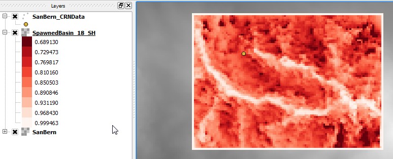
18) from the San Bernardino dataset (viewed in QGIS2.2)12.2.3. Embarrassingly parallel shielding
We provide a python script for running multiple basins using an embarrassingly parallel approach.
It is written for our cluster:
if your cluster uses qsub or equivalent, you will need to write your own script.
However, this will work on systems where you can send jobs directly.
-
To set the system up for embarrassingly parallel runs, you need to run the python script
ManageShieldingComputation.py, which can be found here: https://github.com/LSDtopotools/LSDAutomation. You can download it with:$ wget https://github.com/LSDtopotools/LSDAutomation/raw/master/ManageShieldingComputation.py -
In
ManageShieldingComputation.py, navigate to the bottom of the script, and enter thepath,prefix, andNJobs.NJobsis the number of jobs into which you want to break up the shielding computation. -
Once you run this computation, you will get files with the extension
_bkNNwhereNNis a job number. -
In addition a text file is generated, with the extension
_ShieldCommandPrompt.txt, and from this you can copy and paste job commands into a Linux terminal.These commands are designed for the GeoSciences cluster at the University of Edinburgh: if you use qsubyou will need to write your own script. -
Note that the parameters for the shielding calculation are in the
.CRNParamfiles. We recommend:theta_step:8 phi_step: 5These are based on extensive sensitivity analyses and balance computational speed with accuracy. Errors will be << 1% even in landscapes with extremely high relief. Our forthcoming paper has details on this.
-
Again, these computations take a long time. Don’t start them a few days before your conference presentation!!
-
Once the computations are finished, there will be a shielding raster for every spawned basin raster. In addition, the
_CRNRasters.csvfile will be updated to reflect the new shielding rasters so that the updated parameter files can be fed directly into the erosion rate calculators.
12.2.4. Once you have finished with spawning and topographic shielding calculations
If you are not going to assimilate reported snow shielding values, you can move on to the erosion rate calculations. If you are going to assimilate reported snow shielding values, please read the section: Using previously reported snow shielding.
12.2.5. Stand alone topographic shielding calculations
We also provide a stand alone program just to calculate topographic shielding. This may be useful for samples collected for measuring exposure ages or for working in other settings such as active coastlines.
-
You will first need to compile the program that calculates topographic shielding. This can be compiled with:
$ make -f TopoShielding.make -
The compiled program (
TopoShielding.out) takes four arguments: thePATHNAME, thePREFIX, theAZIMUTH STEPand theANGLE STEP. -
You could simply run this on a single CPU; for example if the original DEM had the prefix
CRN_TESTbefore spawning, and you wanted to use anAZIMUTH_STEP=5andANGLE_STEP=5, you could run the program with:$ ./TopoShielding.out PATHNAME CRN_TEST 5 5where
PATHNAMEis the path to yourCRN_TEST.The DEM must be in ENVI *.bil format. See What data does LSDTopoToolbox take?
This will produce a single topographic shielding raster (with _TopoShield in the filename).
12.3. Snow shielding calculations
Snow absorbs cosmic rays and so CRN concentrations in sediments can be affected by snow that has been present in the basin during the period that eroded materials were exposed to cosmic rays.
Estimating snow shielding is notoriously difficult (how is one to rigorously determine the thickness of snow averaged over the last few thousand years?), and our software does not prescribe a method for calculating snow shielding.
Rather, our tools allow the user to set snow shielding in 3 ways:
-
Use a previously reported basinwide average snow shielding factor
-
Assign a single effective average depth of snow over a catchment (in g cm-2).
-
Pass a raster of effective average depth of snow over a catchment (in g cm-2).
12.3.1. Using previously reported snow shielding
Some authors report a snow shielding factor in their publications. The underlying information about snow and ice thickness used to generate the snow shielding factor is usually missing. Because under typical circumstances the spatial distribution of snow thicknesses is not reported, we use reported snow shielding factors to calculate an effective snow thickness across the basin.
This approach is only compatible with our spawning method (see the section on Spawning the basins), because this average snow thickness will only apply to the raster containing an individual sample’s basin.
The effective snow thickness is calculated by:
where \(d_{eff}\) is the effective depth (g cm-2), \(\Gamma_0\) is the attenuation mass (= 160 g cm-2) for spallation (we do not consider the blocking of muons by snow), and, \(S_s\) is the reported snow shielding.
The reported snow shielding values should be inserted as the 8th column in the CRNData.csv file.
For example,
Sample_name,Latitude,Longitude,Nuclide,Concentration,Uncertainty,Standardisation,Snow_shield
20,34.3758,-117.09,Be10,215100,9400,07KNSTD,0.661531836
15,34.3967,-117.076,Be10,110600,7200,07KNSTD,0.027374149
19,34.4027,-117.063,Be10,84200,6500,07KNSTD,0.592583113
17,34.2842,-117.056,Be10,127700,5800,07KNSTD,0.158279369
14,34.394,-117.054,Be10,101100,6100,07KNSTD,0.047741051
18,34.2794,-117.044,Be10,180600,10000,07KNSTD,0.559339639
11,34.1703,-117.044,Be10,7700,1300,07KNSTD,0.210018127
16,34.2768,-117.032,Be10,97300,5500,07KNSTD,0.317260607
10,34.2121,-117.015,Be10,74400,5200,07KNSTD,0.253863843Steps to use reported snow shielding
Reported snow shielding values are done on a basin-by-basin basis, so our snow shielding must have individual shielding calculations for each sample. This is only possible using our "spawning" routines.
-
The spawning of basins must be performed: see Spawning the basins
-
The
*_spawned_CRNData.csvshould have snow shielding values in the 8th column. -
A python script,
JoinSnowShielding.py, must be run that translates reported snow shielding values into effective depths. This script, and a required helper script,LSDOSystemTools.pycan be downloaded from:$ wget https://github.com/LSDtopotools/LSDAutomation/raw/master/JoinSnowShielding.py $ wget https://github.com/LSDtopotools/LSDAutomation/raw/master/LSDOSystemTools.pyYou will need to scroll to the bottom of the
JoinSnowShielding.pyprogram and edit both the path name and the file prefix. For example, if your spawned data was in/home/ExampleDatasets/SanBernardino/and the files wereSanBern_spawned_CRNRasters.csv,SanBern_spawned_CRNData.csv, andSanBern_spawned.CRNParam, then the bottom of the python file should contain:if __name__ == "__main__": path = "/home/ExampleDatasets/SanBernardino" prefix = "SanBern_spawned" GetSnowShieldingFromRaster(path,prefix) -
This script will then modify the
*spawned_CRNRasters.csvso that the second column will have an effective snow shiedling reflecting the reported snow shielding value (converted using the equation earlier in this section). It will print a new file,*spawned_SS_CRNRasters.csvand copy the CRNData and CRNParam files to ones with prefixes:*_spawned_SS_CRNData.csvand*_spawned_SS.CRNParam. -
These new files (with
_SSin the prefix) will then be used by the erosion rate calculator.
12.3.2. Assign a single effective average depth
This option assumes that there is a uniform layer of time-averaged snow thickness over the entire basin. The thickness reported is in effective depth (g cm-2).
To assign a constant thickness, one simply must set the section column of *_CRNRasters.csv file to the appropriate effective depth.
For example, a file might look like:
/home/topodata/SanBern,15
/home/topodata/Sierra,15,0
/home/topodata/Ganga,15,0,/home/topodata/Ganga_shieldedIn the above example the first row just sets a constant effective depth of 15 g cm-2, The second also assigns a self shielding value of 0 g cm-2 (which happens to be the default), and the third row additionally identifies a topographic shielding raster.
In general, assigning a constant snow thickness over the entire DEM is not particularly realistic, and it is mainly used to approximate the snow shielding reported by other authors when they have not made the spatially distributed data about snow thicknesses available see Using previously reported snow shielding.
12.3.3. Pass a raster of effective average depth of snow over a catchment
Our software also allows users to pass a raster of effective snow thicknesses (g cm-2). This is the time-averaged effective thickness of snow which can be spatially heterogeneous.
The raster is given in the second column of the *_CRNRasters.csv, so, for example in the below file the 4th and 6th rows point to snow shielding rasters.
/home//basin_data/Site01/Site01_DEM,0,0,/home/basin_data/Site01/Site01_DEM_TopoShield
/home/basin_data/Site02/Site02_DEM,5,10
/home/basin_data/Site03/Site03_DEM,5,/home/basin_data/Site03/Site03_DEM_SelfShield
/home/basin_data/Site04/Site04_DEM,/home/basin_data/Site04/Site04_DEM_SnowShield,/home/basin_data/Site04/Site04_DEM_SelfShield
/home/basin_data/Site05/Site05_DEM
/home/basin_data/Site06/Site06_DEM,/home/basin_data/Site06/Site06_DEM_SnowShield| The snow shielding raster must be the same size and shape as the underlying DEM (i.e. they must have the same number of rows and columns, same coordinate system and same data resolution). |
| These rasters need to be assigned BEFORE spawning since the spawning process will clip the snow rasters to be the same size as the clipped topography for each basin. |
12.3.4. Compute snow shielding from snow water equivalent data
In some cases you might have to generate the snow shielding raster yourself. We have prepared some python scripts and some C++ programs that allow you to do this.
-
First, you need to gather some data. You can get the data from snow observations, or from reconstructions. The simple functions we have prepared simply approximate snow water equivalent (SWE) as a function of elevation.
-
You need to take your study area, and prepare a file that has two columns, seperated by a space. The first column is the elevation in metres, and the second column is the average annual snow water equivalent in mm. Here is an example from Idaho:
968.96 70.58333333 1211.2 16 1480.692 51.25 1683.568 165.8333333 1695.68 115.4166667 1710.82 154.1666667 1877.36 139.75 1925.808 195.1666667 1974.256 277.75 2240.72 253.0833333 2404.232 241.5833333 2395.148 163.0833333 -
Once you have this file, download the following python script from our repository:
$ wget https://github.com/LSDtopotools/LSDTopoTools_CRNBasinwide/raw/master/SnowShieldFit.py -
Open the python file and change the filenames to reflect the name of your data file withing the python script, here (scroll to the bottom):
if __name__ == "__main__":

    # Change these names to create the parameter file.  The first line is the name
    # of the data file and the second is the name of the parameter file
    filename = 'T:\\analysis_for_papers\\Manny_idaho\\SWE_idaho.txt'
    sparamname = 'T:\\analysis_for_papers\\Manny_idaho\\HarringCreek.sparam'
This script will fit the data to a bilinear function, shown to approximate the SWE distribution with elevation in a number of sites. You can read about the bilinear fit in a paper by Kirchner et al., HESS, 2014 and by Grünewald et al., Cryosphere, 2014.
For reasons we will see below the prefix (that is the pit before the
.sparam) should be the same as the name of the elevation DEM upon which the SWE data will be based. -
Run the script with:
$ python SnowShieldFit.py -
This will produce a file with the extension sparam. The .sparam file contains the slope and intercept for the annual average SWE for the two linear segments, but in units of g cm-2. These units are to ensure the snow water equivalent raster is in units compatible with effective depths for cosmogenic shielding.
The data file you feed in to SnowShieldFit.pyshould have SWE in mm, whereas the snow shielding raster will have SWE in effective depths with units g cm-2. -
Okay, we can now use some C++ code to generate the snow shielding raster. If you cloned the repository (using
git clone https://github.com/LSDtopotools/LSDTopoTools_AnalysisDriver.git), you will have a function for creating a snow shielding raster. Navigate to thedriver_functionsfolder and make the program using:$ make -f SimpleSnowShield.make -
You run this program with two arguments. The first argument is the path to the
.sparamfile that was generated by the scriptSnowShieldFit.py. The path MUST include a final slash (i.e./home/a/directory/will work but/home/a/directorywill fail.) The second argument is the prefix of the elevation DEM AND the.sparamfile (i.e. if the file isHarringCreek.sparamthen the prefix isHarringCreek). The code will then print out anbilformat raster with the prefix plus_SnowBLso for example if the prefix isHarringCreekthen the output raster isHarringCreek_SnowBL.bil. The command line would look something like:$ ./The prefix of the .sparamfile MUST be the same as the DEM prefix. -
Congratulations! You should now have a snow shielding raster that you can use in your CRN-based denudation rate calculations. NOTE: The program
SimpleSnowShield.execan also produce SWE rasters using a modified Richard’s equation, which has been proposed by Tennent et al., GRL, but at the moment we do not have functions that fit SWE data to a Richard’s equation so this is only recommended for users with pre-calculated parameters for such equations. -
If you have performed this step after spawning the DEMs (see the section Spawning the basins), you can update the
_CRNRasters.csvby running the python scriptPrepareCRNRastersFileFromDirectory.py, which you can read about in the section: Modifying your CRNRasters file the python way.
12.4. Calculating denudation rates
Okay, now you are ready to get the denudation rates.
You’ll need to run the function from the directory where the compiled code is located
(in our example, /home/LSDTT_repositories/LSDTopoTools_CRNBasinwide/), but it can work on data in some arbitrary location.
12.4.1. Compiling the code
To compile the code, go to the driver function folder
(in the example, /home/LSDTT_repositories/LSDTopoTools_CRNBasinwide/driver_functions_CRNBasinwide)
and type:
$ make -f Basinwide_CRN.makeThis will result in a program called Basinwide_CRN.exe.
12.4.2. Running the basin averaged denudation rate calculator
$ ./Basinwide_CRN.exe pathname_of_data file_prefix method_flag-
The pathname_of_data is just the path to where your data is stored, in this example that is
/home/ExampleDatasets/SanBernardino/.You MUST remember to put a /at the end of your pathname. -
The filename is the PREFIX of the files you need for the analysis (that is, without the extension). In the example this prefix is
SanBern(orSanBern_Spawnedif you spawned separate shielding basins) -
The
method_flagtells the program what method you want to use to calculate erosion rates. The options are:
| Flag | Description |
|---|---|
0 |
A basic analysis that does not include any shielding (i.e., no topographic, snow or self shielding). |
1 |
An analysis that includes shielding, but does not account for spawning (see Spawning the basins for details on spawning). If this option is used on spawned basins it is likely to result in errors. Note that spawning speeds up calculations if you have multiple processors at your disposal, but |
2 |
An analyis that includes shielding, to be used on spawned basins (see Spawning the basins for details on spawning). This is the default. |
12.4.3. The output files
There are two output files. Both of these files will end up in the pathname that you designated when calling the program.
The first is called file_prefix_CRNResults.csv and the second is called file_prefix_CRONUSInput.txt
where file_prefix is the prefix you gave when you called the program.
So, for example, if you called the program with:
$ ./basinwide_CRN.exe /home/ExampleDatasets/SanBernardino/ SanBernThe outfiles will be called:
SanBern_CRNResults.csv
SanBern_CRONUSInput.txt
The _CRONUSInput.txt is formatted to be cut and pasted directly into the CRONUS calculator.
The file has some notes (which are pasted into the top of the file):
->IMPORTANT nuclide concentrations are not original!
      They are scaled to the 07KNSTD!!
->Scaling is averaged over the basin for snow, self and topographic shielding.
->Snow and self shielding are considered by neutron spallation only.
->Pressure is an effective pressure that reproduces Stone scaled production
      that is calculated on a pixel by pixel basis.
->Self shielding is embedded in the shielding calculation and so
sample thickness is set to 0.| You should only paste the contents of the file below the header into the CRONUS calculator, which can be found here: http://hess.ess.washington.edu/math/al_be_v22/al_be_erosion_multiple_v22.php A new version of the CRONUS caluclator should be available late 2016 but should be backward compatible with the prior version. See here: http://hess.ess.washington.edu/math/index_dev.html |
The _CRNResults.csv is rather long.
It contains the following data in comma separated columns:
| Column | Name | Units | Description |
|---|---|---|---|
1 |
basinID |
Integer |
A unique identifier for each CRN sample. |
2 |
sample_name |
string |
The name of the sample |
3 |
Nuclide |
string |
The name of the nuclide. Must be either |
4 |
latitude |
decimal degrees |
The latitude. |
5 |
longitude |
decimal degrees |
The longitude. |
6 |
concentration |
atoms/g |
The concentration of the nuclide. This is adjusted for the recent standard (e.g., 07KNSTD), so it may not be the same as in the original dataset. |
7 |
concentration_uncert |
atoms/g |
The concentration uncertainty of the nuclide. Most authors report this as only the AMS uncertainty. The concentration is adjusted for the recent standard (e.g., 07KNSTD), so it may not be the same as in the original dataset. |
8 |
erosion rate |
g cm-2 yr-1 |
The erosion rate in mass per unit area: this is from the full spatially distributed erosion rate calculator. |
9 |
erosion rate AMS_uncert |
g cm-2 yr-1 |
The erosion rate uncertainty in mass per unit area: this is from the full spatially distributed erosion rate calculator. The uncertainty is only that derived from AMS uncertainty. |
10 |
muon_uncert |
g cm-2 yr-1 |
The erosion rate uncertainty in mass per unit area derived from muon uncertainty. |
11 |
production_uncert |
g cm-2 yr-1 |
The erosion rate uncertainty in mass per unit area derived from uncertainty in the production rate. |
12 |
total_uncert |
g cm-2 yr-1 |
The erosion rate uncertainty in mass per unit area that combines all uncertainties. |
13 |
AvgProdScaling |
float (dimensionless) |
The average production scaling correction for the basin. |
14 |
AverageTopoShielding |
float (dimensionless) |
The average topographic shielding correction for the basin. |
15 |
AverageSelfShielding |
float (dimensionless) |
The average self shielding correction for the basin. |
16 |
AverageSnowShielding |
float (dimensionless) |
The average snow shielding correction for the basin. |
17 |
AverageShielding |
float (dimensionless) |
The average of combined shielding. Used to emulate basinwide erosion for CRONUS. CRONUS takes separate topographic, snow and self shielding values, but our code calculates these using a fully depth integrated approach so to convert our shielding numbers for use in CRONUS we lump these together to be input as a single shielding value in CRONUS. |
18 |
AvgShield_times_AvgProd |
float (dimensionless) |
The average of combined shielding times production. This is for use in emulating the way CRONUS assimilates data, since it CRONUS calculates shielding and production separately. |
19 |
AverageCombinedScaling |
float (dimensionless) |
The average combined shielding and scaling correction for the basin. |
20 |
outlet_latitude |
decimal degrees |
The latitude of the basin outlet. This can be assumed to be in WGS84 geographic coordinate system. |
21 |
OutletPressure |
hPa |
The pressure of the basin outlet (calculated based on NCEP2 data after CRONUS). |
22 |
OutletEffPressure |
hPa |
The pressure of the basin outlet (calculated based on NCEP2 data after CRONUS) needed to get the production scaling at the outlet. |
23 |
centroid_latitude |
decimal degrees |
The latitude of the basin centroid. This can be assumed to be in WGS84 geographic coordinate system. |
24 |
centroidPressure |
hPa |
The pressure of the basin centroid (calculated based on NCEP2 data after CRONUS). |
25 |
CentroidEffPressure |
hPa |
This is the pressure needed to get basin averaged production scaling: it is a means of translating the spatially distributed production data into a single value for the CRONUS calculator. |
26 |
eff_erate_COSMOCALC |
g cm-2 yr-1 |
The erosion rate you would get if you took production weighted scaling and used cosmocalc. |
27 |
erate_COSMOCALC_mmperkyr_rho2650 |
mm kyr-1 |
The erosion rate you would get if you took production weighted scaling and used cosmocalc. Assumes \(/rho\) = 2650 kg m-3. |
28 |
eff_erate_COSMOCALC_emulating_CRONUS |
g cm-2 yr-1 |
The erosion rate if you calcualte the average shielding and scaling separately (as done in CRONUS) but erosion rate is caluclated using COSMOCALC. Assumes \(/rho\) = 2650 kg m-3. |
29 |
erate_COSMOCALC_emulating_CRONUS_mmperkyr_rho2650 |
mm kyr-1 |
Uncertainty in the erosion rate. Assumes 2650 kg m-2. |
30 |
erate_mmperkyr_rho2650 |
mm kyr-1 |
This is the erosion rate calculated by our full calculator in mm kyr-1 assuming \(/rho\) = 2650 kg m-3. |
31 |
erate_totalerror_mmperkyr_rho2650 |
mm kyr-1 |
Uncertainty in the erosion rate using the full calculator. Assumes \(/rho\) = 2650 kg m-3. |
32 |
basin_relief |
m |
The relief of the basin. Because production scales nonlinearly with elevation, it is likeley that errors in erosion rates arising from not calculating production on a pixel-by-pixel basis will correlate with relief. In addition, higher relief areas will have greater topographic shielding, so prior reported results that used either no topographic shielding or low resoltion topographic shielding are likeley to have greater errors. |
Reducing the output data
Users may wish to reduce the data contained within _CRNResults.csv file, so we provide python scripts for doing so.
12.4.4. Nested basins
Frequently field workers sample drainage basins that are nested within other basins. We can use denudation rate data from nested basins to calculate the denudation rate required from the remainder of the basin to arrive at the measured CRN concentrations.
Our repository contains a function that allows calculation of CRN-derived denudation rates given a mask of known denudation rates. We refer to it as a nesting calculator because we expect this to be its primary use, but because the program takes a known erosion rate raster the known denudation rate data can take any geometry and one can have spatially heterogeneous known denudation rates.
-
If you have checked out the repository, you can make the nesting driver with:
$ make -f Nested_CRN.make -
To run the code, you need a path and a file prefix, just as in with the
Basinwide_CRN.exe. The path MUST include a trailing slash (e.g.,/home/a/directory/and NOT/home/a/directory), and the prefix should point to the_CRNRasters.csv,_CRNData.csv, and.CRNparamfiles. If any of these files are missing from the directory that is indicated in the path argument the code will not work.An example call to the program might look like:
$ ./Nested_CRN.exe /path/to/data/ My_prefix -
For each raster listed in the directory indicated by the path, the
Nested_CRNprogram will look for a raster with the same prefix but with the added string_ERKnown. You MUST have this exact string in the filename, and it is case sensitive. So for example if your raster name isHarringCreek.bilthe know denudation rate raster must be namesHarringCreek_ERKnown.bil. -
The denudation rate raster MUST be in units of g cm-2 yr-1. This raster MUST be the same size as the elevation raster.
-
The data outputs will be the same as in the case of the
Basinwide_CRN.exeprogram.
How do I make an _ERKnown raster?
We leave it up to the user to produce an _ERKnown raster, but we do have some scripts that can make this a bit easier.
We have made a small python package for manipulating raster data called LSDPlottingTools. You can get it in its very own github repository: https://github.com/LSDtopotools/LSDMappingTools, which you can clone (into a seperate folder if I were you) with:
$ git clone https://github.com/LSDtopotools/LSDMappingTools.gitOnce you have cloned that folder, you should also get the LSDOSystemTools.py scripts using
$ wget https://github.com/LSDtopotools/LSDAutomation/raw/master/LSDOSystemTools.pyOnce you have these python scripts, you can take a basin mask (these are generated by Basinwide_CRN.exe) if the option write_basin_index_raster:
is set to True in the .CRNParam file and call the module from the LSDPlottingTools package SetToConstantValue.
For example, you should have a directory that contains the subdirectory LSDPlottingTools and the script LSDOSystemTools.py. Within the directory you could write a small python script:
import LSDPlottingTools as LSDP

def ResetErosionRaster():
    DataDirectory = "T://basin_data//nested//"
    ConstFname = "ConstEros.bil"
    NewErateName = "HarringCreek_ERKnown.bil"
    ThisFile = DataDirectory+ConstFname
    NewFilename = DataDirectory+NewErateName

    LSDP.CheckNoData(ThisFile)

    # now print the constant value file
    constant_value = 0.0084
    LSDP.SetToConstantValue(ThisFile,NewFilename,constant_value)

    LSDP.CheckNoData(NewFilename)

if __name__ == "__main__":
    #fit_weibull_from_file(sys.argv[1])
    #TestNewMappingTools2()
    #ResetErosionRaster()
    #FloodThenHillshade()
    FixStupidNoData()
This script resets any raster data that is not NoData to the value denoted by constant_value so cannot produce spatially heterogeneous denudation rates: for that you will need to write your own scripts.
12.4.5. Soil or point data
CAIRN is also capable of calculating the denudation rates from soil or point samples. Online calculators such as the CRONUS calculator can calculate denudation rates at a single site but some users who have both basinwide and soil sample may wish to calculate both denudation rates with CAIRN for consistency.
The user inputs and outputs for the soil samples are similar to thos of the basin average scripts.
-
The
_CRNRasters.csvfile should have the same format as for basinwide samples. -
The
_CRNData.csvfile should have the same format as for basinwide samples. -
The
.CRNParamfile should have the same format as for basinwide samples
However, and additional file is needed with the extention _CRNSoilInfo.csv. This file needs to have the same prefix as the other parameter files.
The format of this file is:
| Column | Name | Units | Description |
|---|---|---|---|
1 |
sample_top_depth_cm |
string |
The sample names need to be the same as in the |
2 |
sample_top_depth_cm |
cm |
The depth of the top of the sample in cm. |
3 |
sample_bottom_depth_cm |
cm |
The depth of the bottom of the sample in cm. |
4 |
density_kg_m3 |
kg m-3 |
The density of the sample. Note that this assumes that everything above the sample is the same density. These are converted into effective depths so if denisty is varying users should use some default denisty (e.g., 2000 kg m-2) and then enter depths in cm the, when multiplied by the density, will result in the correct effective depth. |
An example file looks like this:
sample_name,sample_top_depth_cm,sample_bottom_depth_cm,density_kg_m3
S1W-Idaho,0,2,1400
S2W-Idaho,0,2,1400
S3W-Idaho,0,2,1400
To run the soil calculator, you need to compile the soil calculator that is include in the repository:
$ make -f Soil_CRN.makeAnd then run the code including the path name and the prefix of the data files, for example:
$ ./Soil_CRN.exe /home/smudd/SMMDataStore/analysis_for_papers/Manny_idaho/Revised/Soil_Snow/ HarringCreek_Soil_SnowShield12.5. Summary
You should now be able to take concentrations from detrital cosmogenics and convert these into basin averaged denudation rates.
: numbered :
13. Swath Profiling Tools
| These tools have extra dependencies in addition to a standard installation of LSDTopoTools. Make sure you have read the requirements overview section and installed the libraries needed to run these tools. Detailed installation information is also found in the appendix. |
13.1. Generalised Swath Profile
Here we expain how to generate a generalised swath profile following the same algorithm described by Hergarten et al. (2014).
The outputs from the function are:
-
A raster showing the extent of the swath profile, indicating the perpendicular distance of each point from the baseline (i.e. a transverse swath)
-
A raster showing the extent of the swath profile, indicating the projected distance along the baseline (i.e. a longitudinal swath)
-
A
.txtfile containing the results of the transverse swath profile. The table includes the distance of the centre of each bin across the profile, the mean and standard deviation of each bin, and the 0, 25, 50, 75 and 100 percentiles. -
A
.txtfile containing the results of the longitudinal swath profile. The table includes the distance of the centre of each bin along the profile, projected onto the baseline, the mean and standard deviation of each bin, and the 0, 25, 50, 75 and 100 percentiles.
In order to do so, there are a few preprocessing steps that need to be done to generate the profile baseline. These can easily be done in ArcMap, but the experienced LSDTopotools user can also write a more complex driver function to do more specialised tasks.
13.1.1. Preprocessing step 1: Getting your raster into the correct format
You will need to get data that you have downloaded into a format LSDTopoToolbox can understand, namely the .flt format.
13.1.2. Preprocessing step 2: Creating the baseline
| This step can be done automatically by tweaking the driver file to extract the baseline using the LSDTopoTools package. See Channel Long Profile Swaths a few sections below for an example of this, which avoids using the pesky ArcMap software. |
The baseline is the centre line of the swath profile. At present the SwathProfile tool uses a shapefile *.shp consisting of a series of points that define the profile. A suitable baseline can be produced in two easy steps.
-
First, create a new shapefile, setting the feature class to
polyline, and create a single line feature, which will form the baseline. This can be linear, or curved, depending on what your requirements are. Next create another shapefile, this time make the feature classpoint.
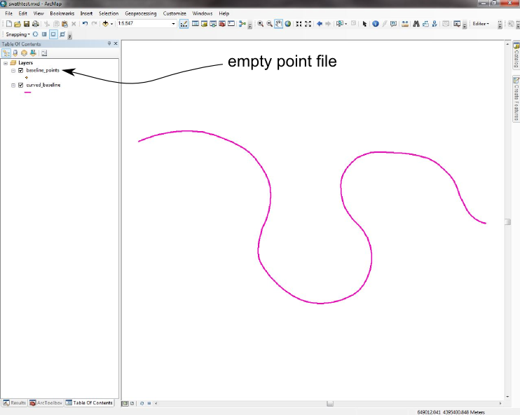
-
Start editing in ArcMap. Make the target class the new, empty
pointshapefile. Using the edit tool on the Editor Toolbar, select the polyline that you drew in the previous step; it should be highlighted in a light blue colour. Go to the drop-down menu on the Editor toolbar, and select "Construct Points…". Set the template as the emptypointshapefile. Set the construction option to Distance, and make the point spacing equal to the resolution of your DEM. Make sure "Create additional points at start and end" is checked. Click ok, then save your edits… you have now created the baseline file. Give yourself a pat on the back, take a deep breath and move onto the next stage…
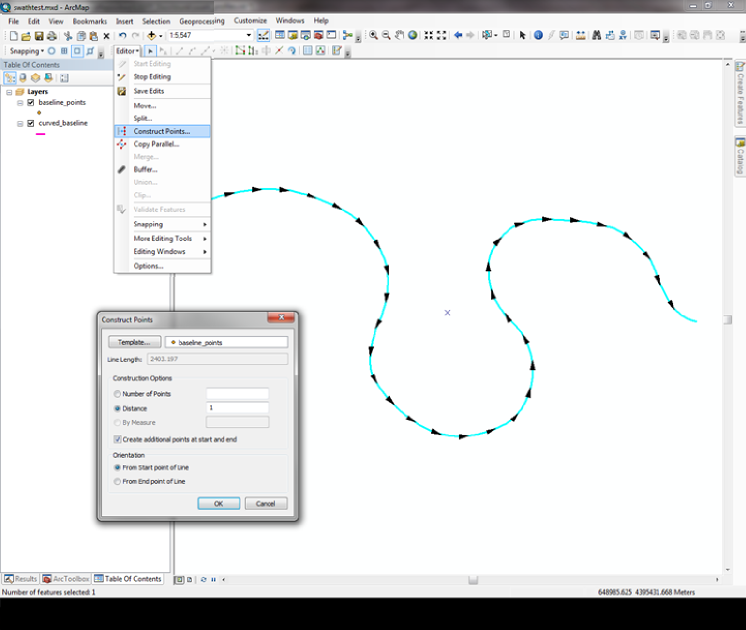
13.1.3. Compiling the driver function
You will need to download all of the code. This will have a directory with the objects (their names start with LSD). Note that this tool utilises the PCL library: PCL homepage. Hopefully this is already installed on your University server (it is on the University of Edinburgh server). It probably won’t be installed on your laptop, unless you have installed it yourself at some point. This tool will not work if the PCL library is not installed!
Within the directory with the objects, there will be two additional directories:
-
driver_functions
-
TNT
The TNT folder contains routines for linear algebra, and it is made by NIST, you can happily do everything in
LSDTopoToolbox without ever knowing anything about it, but if you want you can read what it is here: TNT homepage.
In order to compile this function, it is necessary to use cmake (version 2.8 or later). The compilation procedure is as follows:
-
First, go into the driver function folder
-
Make a new directory in this folder named
build; in your terminal type:
mkdir build-
Move the
CMakeLists_SwathProfile.txtfile into thebuilddirectory. At the same time, rename this fileCMakeLists.txt, so the compiler will find it. Type::
mv CMakeLists_SwathProfile.txt build/CMakeLists.txt-
Go into the
builddirectory. Type:
cmake28 .in the terminal. Note that the name of this directory isn’t important.
-
Next type:
makein the terminal. This compiles the code. You will get a bunch of messages but at the end your code will have compiled.
-
All that is left to do is to move the compiled function back up into the driver_functions directory. Type:
mv swath_profile_driver.out ..13.1.4. Running the driver function
Okay, now you are ready to run the driver function. You’ll need to run the function from the directory where the compiled code is located (i.e. the driver_functions folder), but it can work on data that is located in any location.
-
You run the code with the command
./swath_profile_driver.out name_of_basline_file name_of_raster half_width_of_profile bin_width_of_profile -
The
name_of_baseline_fileis just the name of the shapefile created in the preprocessing step that contains the points defining the baseline. -
The
name_of_rasteris the PREFIX of the raster, so if your raster is calledlat_26p5_flt.fltthen thename_of_rasterislat_26p5_flt(that is, without the.fltat the end). -
Note that if your data is stored in a
differentdirectory, then you will need to inlude the full path name inname_of_rasterandname_of_baseline_file. The output files will be saved in the same directory as the DEM. -
The
half_width_of_profileis the half width of the swath (i.e. the distance from the baseline to the swath edge). -
The
bin_width_of_profileis the resolution at which the profile data is condensed into a single profile. This is not the same as the raster resolution!
13.1.5. Program outputs
The swath_profile_driver tool creates two raster datasets, so you can check the swath templates yourself to better understand how the profiles are constructed
-
*_swath_long.fltis the longitudinal swath profile template
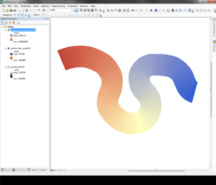
-
*_swath_trans.fltis the transverse swath profile template
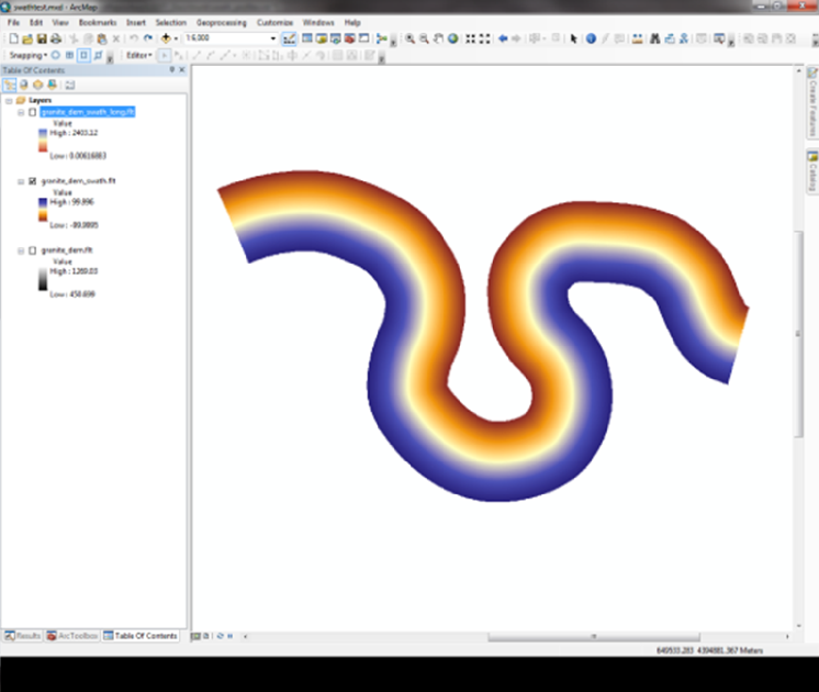
There are also two .txt files, which contain the profile data → these include the mean, standard deviation, and percentiles for each. These can be plotted using the python script plot_swath_profile.py, located in the LSDVisualisation/trunk/ directory.
13.2. Channel Long Profile Swaths
Here another use of the swath tools feature is exploited. You can use it to automatically create long profiles along a channel using a value other than elevation, for example. (This usage is hinted at in the Hergarten et al. (2014) paper. This application is mainly suited to where there is:
-
Expected to be some variation along channel of a certain value or other metric
-
The DEM resolution is high enough to capture lateral variations across the channel, but you are interested in the average of these metrics along the long profile.
13.2.1. Example Applications
-
Channel width variation using high resolution lidar DEMs
-
Sediment size distribution along channel from model output
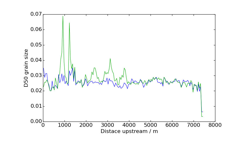
-
Erosion/deposition distribution along channel from model output
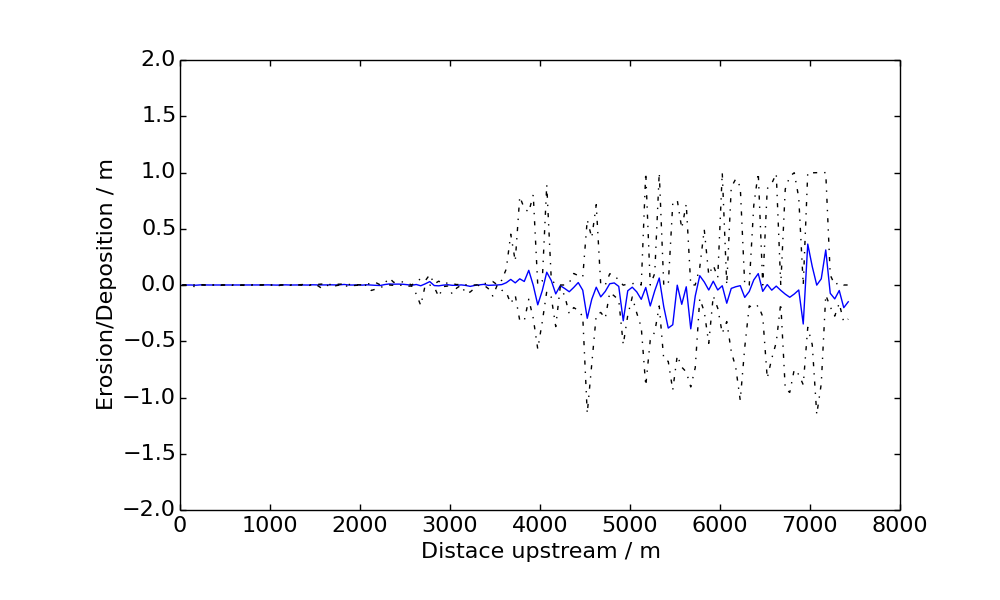
-
Basin hydrology applications (water depth, velocity etc.)
You will need the driver file: longitudinal_channel_erosion_swath_profiler.cpp along with the corresponding CMake file.
There are effectively 3 supplementary files you need to perform this analysis.
-
Parameter file. This takes the form of a simple text file with a column of values:
-
Terrain DEM Name (The base topography)
-
Secondary Raster/DEM file name. (This is the raster file that contains the property that varies along channel.)
-
Raster extension for the above two files (currently, both must be the same format)
-
Minslope (use 0.00001 for starters)
-
Contributing pixel threshold (for calculating the drainage network
-
Swath Half Width (see above)
-
Swath Bin Width (see above)
-
Starting Junction Number
-
-
Terrain Raster
-
Secondary Raster
These two rasters should be in the same spatial extent.
13.2.2. Example Usage
Compile the driver file using CMake. To do this, create a build folder in the driver_functions folder. Copy the file CMakeLists_Swath_long_profile_erosion.txt file into the new folder, and rename it CMakeLists.txt, as described above. Then:
cmake .
make
You now have the executable long_swath_profile_erosion.exe. It is run by giving it two arguments: the path to the parameter file and raster file (in the same directory as each other, but can be separate from the executable) and the name of the parameter file.
./long_swath_profile_erosion.exe ./ swath_profiler_long.paramThe driver file is designed to perform the whole operation in one go: Fill DEM > Extract Channel Network > Produce Channel File > Convert Channel file to X,Y Points for Swath > Create Swath Template > Perform Swath Analysis, but you may want to split it up into stages if you do not know the starting junction number where you want the profile to begin.
The driver file currently uses the longest channel in the basin (the mainstem) so check that this is what you expected. An option may become available to look at tributaries later on.
The output files are the Profile (txt) and the Swath template that was used to profile the channel. (Check that it was the spatial extent that you expected).
You can use the same visualisation script as above: plot_swath_profile.py, located in the LSDVisualisation/trunk/ directory.
14. Floodplain and terrace extraction using channel relief and slope thresholds
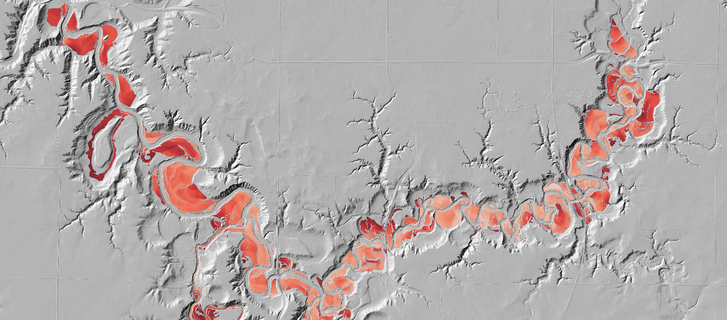
These tools have extra dependencies in addition to a standard installation of LSDTopoTools. If you are using our vagrant distribution with LSDTopoToolsSetup.py then these should be installed for you with the floodplain and terrace code. If not, make sure you have read the requirements overview section and installed the libraries needed to run these tools. Detailed installation information is also found in the appendix.
|
This chapter outlines a method of extracting floodplains and terraces across the landscape based on thresholds of local gradient and elevation compared to the nearest channel. These thresholds are calculated statistically from the DEM using quantile-quantile plots, and do not need to be set manually by the user for the lansdcape in question. For more details on the methodology please refer to Clubb et al. (2017).
Floodplains are extracted across the whole DEM using thresholds of local gradient and relief relative to the nearest identified channel pixel. Terraces are extracted along a channel swath profile using an algorithm developed by Hergarten et al. (2014). The user needs to provide a CSV file with a pair of latitude and longitude coordinates. The code will extract the channel network between these coordinates and identify all terraces along this baseline channel.
14.1. The methodology
The method has several steps, which are outlined below:
-
The DEM is filtered using a Perona-Malik filter, a non-linear filter. For more details please refer to Perona and Malik (1990). This filter was chosen as it reduces micro-topographic noise while preserving sharp boundaries, such as between hillslopes and floodplains.
-
After filtering, the local slope and relief relative to the nearest channel are calculated for each pixel. To calculate the relief relative to the channel, a threshold stream order must be set to ensure that small first order tributaries are not selected. If identifying terraces, relief is calculated based on a swath profile rather than on the nearest channel.
-
Thresholds for slope and channel relief are calculated statistically from the DEM using quantile-quantile plots. This involves plotting the probability density function of each metric and calculating the deviation away from a reference normal distribution.
-
Any pixel with a value lower than both the channel relief and slope threshold is then classified as floodplain or terrace, giving a binary mask of 1 (floodplain/terrace) and 0 (not floodplain/terrace).
-
Floodplains and terraces are separated using a connected components algorithm (He et al. (2008)). Any patches which are connected to the channel network are identified as floodplain. The user can also specify a minimum height of the terraces above the modern channel. The connected components algorithm also assigns a unique ID to each floodplain/terrace.
-
The user can specify various topographic metrics to calculate for each patch of floodplain or terrace, such as elevation compared to the channel.
| This method is in development. We cannot guarantee a bug-free experience! |
14.2. Get the code for floodplain and terrace extraction
The code for floodplain/terrace extraction can be found in our GitHub repository. This repository contains code for identifying floodplains based on relief relative to the nearest channel, and getting terraces along a channel swath profile.
14.2.1. Getting the code using LSDTopoToolsSetup.py
14.2.2. Clone the GitHub repository (not needed if you used LSDTopoToolsSetup.py)
If you haven’t run our vagrant setup, you need to clone the repository. First navigate to the folder where you will keep the GitHub repository. In this example it is called /LSDTopoTools/Git_projects/. To navigate to this folder in a UNIX terminal use the cd command:
$ cd /LSDTopoTools/Git_projects/You can use the command pwd to check you are in the right folder. Once you are in this folder, you can clone the repository from the GitHub website:
$ pwd
/LSDTopoTools/Git_projects/
$ git clone https://github.com/LSDtopotools/LSDTopoTools_FloodplainTerraceExtraction.git
14.2.3. Alternatively, get the zipped code
If you don’t want to use git, you can download a zipped version of the code:
$ pwd
/LSDTopoTools/Git_projects/
$ wget https://github.com/LSDtopotools/LSDTopoTools_FloodplainTerraceExtraction/archive/master.zip
$ gunzip master.zip
GitHub zips all repositories into a file called master.zip,
so if you previously downloaded a zipper repository this will overwrite it.
|
14.2.4. Install the Point Cloud Library
If you aren’t working on our vagrant system, you will need to make sure that you have the Point Cloud Library installed. You can do this on Linux using the apt-get command:
$ sudo add-apt-repository ppa:v-launchpad-jochen-sprickerhof-de/pcl
$ sudo apt-get update
$ sudo apt-get install libpcl-all
Ubuntu 16.04 LTS
If you are using ubuntu 16.04, the above commands won’t work as the repository is broken. You can install the pcl library using the following steps:
Install oracle-java8-jdk:
$ sudo add-apt-repository -y ppa:webupd8team/java && sudo apt update && sudo apt -y install oracle-java8-installerInstall various dependencies and pre-requisites:
$ sudo apt -y install g++ cmake cmake-gui doxygen mpi-default-dev openmpi-bin openmpi-common libusb-1.0-0-dev libqhull* libusb-dev libgtest-dev
$ sudo apt -y install git-core freeglut3-dev pkg-config build-essential libxmu-dev libxi-dev libphonon-dev libphonon-dev phonon-backend-gstreamer
$ sudo apt -y install phonon-backend-vlc graphviz mono-complete qt-sdk libflann-dev libflann1.8 libboost1.58-all-dev

$ cd ~/Downloads
$ wget http://launchpadlibrarian.net/209530212/libeigen3-dev_3.2.5-4_all.deb
$ sudo dpkg -i libeigen3-dev_3.2.5-4_all.deb
$ sudo apt-mark hold libeigen3-dev

$ wget http://www.vtk.org/files/release/7.1/VTK-7.1.0.tar.gz
$ tar -xf VTK-7.1.0.tar.gz
$ cd VTK-7.1.0 && mkdir build && cd build
$ cmake ..
$ make
$ sudo make install
Install Point Cloud Library v1.8:
$ cd ~/Downloads
$ wget https://github.com/PointCloudLibrary/pcl/archive/pcl-1.8.0.tar.gz
$ tar -xf pcl-1.8.0.tar.gz
$ cd pcl-pcl-1.8.0 && mkdir build && cd build
$ cmake ..
$ make
$ sudo make install
Do some clean up:
$ cd ~/Downloads
$ rm libeigen3-dev_3.2.5-4_all.deb VTK-7.1.0.tar.gz pcl-1.8.0.tar.gz
$ sudo rm -r VTK-7.1.0 pcl-pcl-1.8.0
You should now have pcl installed on your system! You can do a small test of the installation if you want to:
$ cd ~
$ mkdir pcl-test && cd pcl-test
Create a CMakeLists.txt file and save this in the directory pcl-test:
cmake_minimum_required(VERSION 2.8 FATAL_ERROR)
project(pcl-test)
find_package(PCL 1.2 REQUIRED)

include_directories(${PCL_INCLUDE_DIRS})
link_directories(${PCL_LIBRARY_DIRS})
add_definitions(${PCL_DEFINITIONS})

add_executable(pcl-test main.cpp)
target_link_libraries(pcl-test ${PCL_LIBRARIES})

SET(COMPILE_FLAGS "-std=c++11")
add_definitions(${COMPILE_FLAGS})
Create a file and call it main.cpp:
#include <iostream>

int main() {
    std::cout << "hello, world!" << std::endl;
    return (0);
}
Compile the cpp file and then test it :
$ mkdir build && cd build
$ cmake ..
$ make
$ ./pcl-test
Output should be hello, world!
14.2.5. Install a couple of other libraries
You might find you need to install a couple of other libraries for the floodplain and terrace drivers to compile properly. If you are using Ubuntu, you can do this using the following commands:
$ sudo apt-get update
$ sudo apt-get install libgoetiff-dev
$ sudo apt-get install liblas-dev
14.3. Preliminary steps
14.3.1. Getting the channel head file
Before the floodplain/terrace extraction algorithm can be run, you must create a channel network for your DEM. This can be done using the Channel extraction algorithms within LSDTopoTools. There are several channel extraction algorithms which you can choose from: for more details please refer to the Channel extraction section. Once you have run the channel extraction algorithm, you must make sure that the csv file with the channel head locations is placed in the same folder as your DEM.
14.3.2. Finding the correct window size
Before we can run the floodplain/terrace extraction algorithm, we need to calculate the correct window size for calculating slope across the DEM. This is used to calculate the thresholds for floodplain/terrace identification. Please refer to the Selecting A Window Size section for information on how to calculate a window size for your DEM. We suggest a value of around 6 m for 1 m resolution DEMs, and a value of 15 m for 10 m resoluton DEMs.
14.4. Floodplains
This section explains how to extract floodplains across the DEM. We have provided some example datasets which you can use in order to test the floodplain extraction. If you are using the vagrant distribution, we recommend that you create a new directory in the Topographic_projects directory for each field site that you analyse. Navigate to the Topographic_projects directory using the cd command:
$ pwd
/LSDTopoTools/Git_projects/
$ cd ..
$ cd Topographic_projects/
In this tutorial we will work using a LiDAR dataset from Mid Bailey Run, Ohio. You should make a new directory for the Mid Bailey Run DEM in the Topographic_projects directory:
$ mkdir Mid_Bailey_Run/
$ cd Mid_Bailey_Run/
You can get the DEM for Mid Bailey Run from our ExampleTopoDatasets repository using wget:
$ wget https://github.com/LSDtopotools/ExampleTopoDatasets/raw/master/Bailey_DEM.bil
$ wget https://github.com/LSDtopotools/ExampleTopoDatasets/raw/master/Bailey_DEM.hdr
This dataset is already in the preferred format for use with LSDTopoTools (the ENVI bil format). The figure below shows a shaded relief map of part of the South Fork Eel River DEM which will be used in these examples.
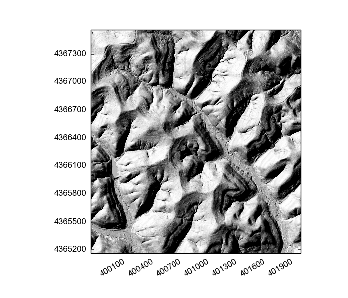
14.4.1. Get the example parameter files
We have also provided some examples parameter files that are used to run the floodplain delineation. You can get the example floodplain driver using wget:
$ wget https://github.com/LSDtopotools/ExampleTopoDatasets/tree/master/example_parameter_files/ExampleFiles_FloodplainTerraceExtraction/LSDTT_floodplains.paramThis should be placed in the same folder as your DEM and the channel heads csv file. The example from Mid Bailey Run is called LSDTT_floodplains.param and should look like this:
# This is a driver file for LSDTopoTools
# Any lines with the # symbol in the first row will be ignored

# File information
dem read extension: bil
dem write extension: bil
read path: /LSDTopoTools/Topographic_projects/Mid_Bailey_Run/
read fname: Bailey_DEM
write fname: Bailey_DEM
CHeads_file: Bailey_DEM_Wsources

# Parameters for floodplain extraction
Filter topography: true
Min slope filling: 0.0001
surface_fitting_window_radius: 6
Threshold_SO: 3
Relief lower percentile: 25
Relief upper percentile: 75
Slope lower percentile: 25
Slope upper percentile: 75
QQ threshold: 0.005
Min patch size: 1000
You can run the analysis on the Mid Bailey Run DEM using the example parameter file, and modify it as you wish for your own DEM.
| You must make sure the description of the parameter in your file matches EXACTLY to the example, or the code will not recognise the parameter properly. If in doubt, check your spelling. |
The table below explains the function of each of these parameters:
| Parameter name | Data type | Description |
|---|---|---|
dem read extension |
String |
The file extension of your input DEM |
dem write extension |
String |
The file extension of the output rasters |
read path |
String |
The path to your DEM and parameter file |
read fname |
String |
The name of your DEM without extension |
CHeads_file |
String |
The name of the channel heads csv file without extension |
Filter topography |
Boolean |
Switch to run the filtering and filling of the DEM. Only set to false if you want to re-run the analysis (to save time). |
Min slope filling |
float |
Minimum slope for filling the DEM, suggested to be 0.0001 |
surface_fitting_window_radius |
float |
Window radius for calculating slope, should be calculated using the window size routines |
Threshold_SO |
integer |
Threshold Strahler stream order for the nearest channel. A value of 3 should work in most landscapes. |
Relief lower percentile |
integer |
Lower percentile for fitting Gaussian distribution to relief from quantile-quantile . Leave as 25 unless you have a weird quantile-quantile plot for the landscape. |
Relief upper percentile |
integer |
Upper percentile for fitting Gaussian distribution to relief from quantile-quantile plots. Leave as 75 unless you have a weird quantile-quantile plot for the landscape. |
Slope lower percentile |
integer |
Lower percentile for fitting Gaussian distribution to slope from quantile-quantile plots. Leave as 25 unless you have a weird quantile-quantile plot for the landscape. |
Slope upper percentile |
integer |
Upper percentile for fitting Gaussian distribution to rslope from quantile-quantile plots. Leave as 75 unless you have a weird quantile-quantile plot for the landscape. |
QQ threshold |
float |
Threshold for calculating difference between the real and Gaussian distributions from the quantile-quantile plots. Leave as 0.005 unless you have a weird quantile-quantile plot for the landscape. |
Min patch size |
integer |
Minimum number of pixels for each floodplain patch, can use to remove very small patches which may be due to noise. |
14.4.2. If you used LSDTopoToolsSetup.py
Navigate to driver_functions_Floodplains-Terraces directory in the folder LSDTopoTools_FloodplainTerraceExtraction:
$ cd /LSDTopoTools/Git_projects/LSDTopoTools_FloodplainTerraceExtraction/driver_functions_Floodplains-Terraces/You have already compiled the code, so you can just run the program with:
$ ./get_floodplains.out /path/to/DEM/location/ name_of_parameter_file.paramFor our example, the command would be:
$ ./get_floodplains.out /LSDTopoTools/Topographic_projects/Eel_River/ LSDTT_floodplains.param14.4.3. If you didn’t use LSDTopoToolsSetup.py
Before the code can be run, you must compile it. To do this you need to go to the driver_functions_Floodplains-Terraces directory in the folder LSDTopoTools_FloodplainTerraceExtraction. Navigate to the folder using the command:
$ cd /LSDTopoTools/Git_projects/LSDTopoTools_FloodplainTerraceExtraction/driver_functions_Floodplains-Terraces/and compile the code with:
$ make -f get_floodplains.makeThis may come up with some warnings, but should create the file get_floodplains.out. You can then run the program with:
$ ./get_floodplains.out /path/to/DEM/location/ name_of_parameter_file.paramFor our example, the command would be:
$ ./get_floodplains.out /LSDTopoTools/Topographic_projects/Eel_River/ LSDTT_floodplains.param14.4.4. Analysing the results
The program should take between 10 - 40 minutes to run, depending on the size of your DEM and your processing power. Once it is completed, you will have a number of bil files which you can open in a GIS of your choice. These files will include:
-
DEM_name_filtered.bil and .hdr: The original DEM after Perona-Malik filtering
-
DEM_name_channel_relief.bil and .hdr: A raster of elevations compared to the nearest channel
-
DEM_name_slope.bil and .hdr: A raster of local gradient
-
DEM_name_qq_relief.txt and _qq_slope.txt: Text files with the quantile-quantile plot information. This can be plotted in our python script to check whether the thresholds selected were appropriate.
-
DEM_name_FP.bil and .hdr: A raster of floodplain locations.
An example of the floodplains extracted from the Mid Bailey Run catchment is shown below. You should be able to get a raster similar to this by opening the file Bailey_DEM_FP.bil in a GIS of your choice.
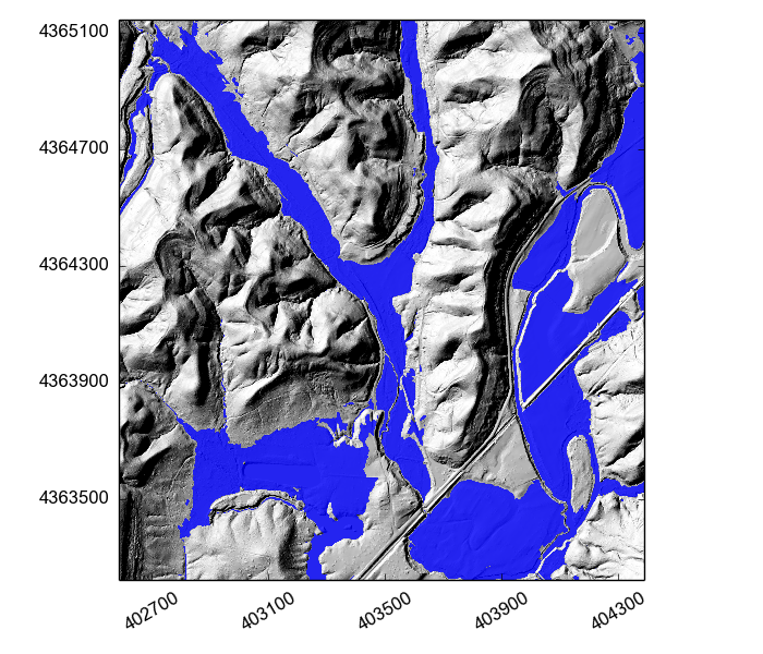
14.5. Terraces
This section explains how to extract terraces along a channel by providing coordinates specifying the upstream and downstream extent of the channel. We have provided some example datasets which you can use in order to test the terrace extraction. If you are using the vagrant distribution, we recommend that you create a new directory in the Topographic_projects directory for each field site that you analyse. Navigate to the Topographic_projects directory using the cd command:
$ pwd
/LSDTopoTools/Git_projects/
$ cd ..
$ cd Topographic_projects/
In this tutorial we will work using a LiDAR dataset from the South Fork Eel River, California. You should make a new directory for the Eel River DEM in the Topographic_projects directory:
$ mkdir Eel_River/
$ cd Eel_River/
You can get the DEM for the South Fork Eel River from our ExampleTopoDatasets repository using wget:
$ wget https://github.com/LSDtopotools/ExampleTopoDatasets/raw/master/Eel_River_DEM.bil
$ wget https://github.com/LSDtopotools/ExampleTopoDatasets/raw/master/Eel_River_DEM.hdr
This dataset is already in the preferred format for use with LSDTopoTools (the ENVI bil format). The figure below shows a shaded relief map of part of the South Fork Eel River DEM which will be used in these examples.
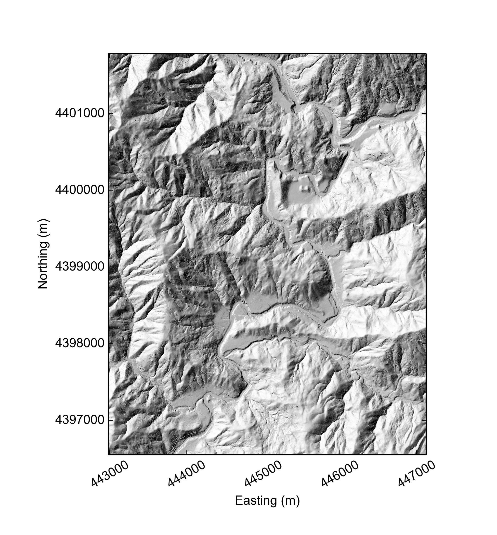
14.5.1. Get the example files
We have also provided two example files that are used to run the terrace extraction. The first is a parameter file that is used to run the code, and the second is a csv file with the latitude and longitude of two points on the Eel River. You can get the example files using wget:
$ wget https://github.com/LSDtopotools/ExampleTopoDatasets/tree/master/example_parameter_files/ExampleFiles_FloodplainTerraceExtraction/LSDTT_terraces.param
$ wget https://github.com/LSDtopotools/ExampleTopoDatasets/tree/master/example_parameter_files/ExampleFiles_FloodplainTerraceExtraction/Eel_River_DEM_coordinates.csv
Make sure that these files are stored in the same place as the DEM!! This should be in the folder /LSDTopoTools/Topographic_projects/Eel_River/
14.5.2. Creating the parameter file
In order to run the terrace extraction code you must first create a parameter file for your DEM. If you have been following this tutorial, you should have downloaded an example parameter file for the Eel River DEM and placed this in the same folder as your DEM and the channel heads csv file. The example from the Eel River is called LSDTT_Swath.param and should look like this:
# This is a driver file for LSDTopoTools
# Any lines with the # symbol in the first row will be ignored

# File information
dem read extension: bil
dem write extension: bil
read path: /LSDTopoTools/Topographic_projects/Eel_River/
read fname: Eel_River_DEM
CHeads_file: Eel_River_DEM_Wsources
coords_csv_file: Eel_River_DEM_coordinates.csv

# Parameters for DEM processing
Filter topography: true
Min slope filling: 0.0001
surface_fitting_window_radius: 6

# Parameters for swath post-processing
HalfWidth: 1000
search_radius: 10
Threshold_SO: 3
NormaliseToBaseline: 1

# Pararmeters for terrace extraction
QQ threshold: 0.005
Relief lower percentile: 25
Relief upper percentile: 75
Slope lower percentile: 25
Slope upper percentile: 75
Min patch size: 1000
Min terrace height: 5
You can run the analysis on the Eel River DEM using the example parameter file, and modify it as you wish for your own DEM.
| You must make sure the description of the parameter in your file matches EXACTLY to the example, or the code will not recognise the parameter properly. If in doubt, check your spelling. |
The table below explains the function of each of these parameters:
| Parameter name | Data type | Description |
|---|---|---|
dem read extension |
String |
The file extension of your input DEM |
dem write extension |
String |
The file extension of the output rasters |
read path |
String |
The path to your DEM and parameter file |
read fname |
String |
The name of your DEM without extension |
CHeads_file |
String |
The name of the channel heads csv file without extension |
coords_csv_file |
String |
The name of the csv file with the coordinates to extract the terraces (must end in .csv) |
Filter topography |
Boolean |
Switch to run the filtering and filling of the DEM. Only set to false if you want to re-run the analysis (to save time). |
Min slope filling |
float |
Minimum slope for filling the DEM, suggested to be 0.0001 |
surface_fitting_window_radius |
float |
Window radius for calculating slope, should be calculated using the window size routines |
HalfWidth |
integer |
Width of the swath profile in metres |
search_radius |
integer |
Number of pixels to search around input latitude/longitude coordinates for the nearest channel. |
Threshold_SO |
integer |
Threshold Strahler stream order for the baseline channel. A value of 3 should work in most landscapes. |
NormaliseToBaseline |
integer |
Switch to normalise the elevations to the nearest channel. For terrace extraction this should always be set to 1. |
QQ threshold |
float |
Threshold for calculating difference between the real and Gaussian distributions from the quantile-quantile plots. Leave as 0.005 unless you have a weird quantile-quantile plot for the landscape. |
Relief lower percentile |
integer |
Lower percentile for fitting Gaussian distribution to relief from quantile-quantile . Leave as 25 unless you have a weird quantile-quantile plot for the landscape. |
Relief upper percentile |
integer |
Upper percentile for fitting Gaussian distribution to relief from quantile-quantile plots. Leave as 75 unless you have a weird quantile-quantile plot for the landscape. |
Slope lower percentile |
integer |
Lower percentile for fitting Gaussian distribution to slope from quantile-quantile plots. Leave as 25 unless you have a weird quantile-quantile plot for the landscape. |
Slope upper percentile |
integer |
Upper percentile for fitting Gaussian distribution to rslope from quantile-quantile plots. Leave as 75 unless you have a weird quantile-quantile plot for the landscape. |
Min patch size |
integer |
Minimum number of pixels for each terrace, can use to remove very small patches which may be due to noise. |
Min terrace height |
integer |
Threshold height for terraces above the channel to separate from modern floodplain. |
14.5.3. Getting the latitude and longitude coordinates
To run the code, you need to provide a CSV file with two pairs of coordinates which specify the upstream and downstream points between which you want to find the terraces. The easiest way to do this is on Google Earth.
We have written the code so that it will take the coordinates in latitude and longitude and automatically convert them to the same UTM zone as the DEM - you don’t need to do this yourself! If you are following the tutorial for the Eel River site, then you should have downloaded the file Eel_River_DEM_coordinates.csv and placed this in the same folder as your DEM. For example, the Eel River file has the following structure:
Point_ID,latitude,longitude
1,39.722956,-123.650299
2,39.754546,-123.631409| The first point in the csv file must be the upstream point and the second point must be the downstream point. If this isn’t the case then the code will break! |
14.5.4. If you used LSDTopoToolsSetup.py
Navigate to the folder driver_functions_Floodplains-Terraces directory in the folder LSDTopoTools_FloodplainTerraceExtraction:
$ cd /LSDTopoTools/Git_projects/LSDTopoTools_FloodplainTerraceExtraction/driver_functions_Floodplains-Terraces/You have already compiled the code, so you can just run the program with:
$ ./get_terraces.out /path/to/DEM/location/ name_of_parameter_file.paramFor our example, the command would be:
$ ./get_terraces.out /LSDTopoTools/Topographic_projects/Eel_River/ LSDTT_terraces.param14.5.5. If you didn’t use LSDTopoToolsSetup.py
Before the code can be run, you must compile it. To do this you need to go to the driver_functions_Floodplains-Terraces directory in the folder LSDTopoTools_FloodplainTerraceExtraction. Navigate to the folder using the command:
$ cd /LSDTopoTools/Git_projects/LSDTopoTools_FloodplainTerraceExtraction/driver_functions_Floodplains-Terraces/and compile the code with:
$ bash get_terraces.shThis may come up with some warnings, but should create the file get_terraces.out. You can then run the program with:
$ ./get_terraces.out /path/to/DEM/location/ name_of_parameter_file.paramFor our example, the command would be:
$ ./get_terraces.out /LSDTopoTools/Topographic_projects/Eel_River/ LSDTT_terraces.param14.5.6. Analysing the results
The program should take between 10 - 40 minutes to run, depending on the size of your DEM and your processing power. Once it is completed, you will have a number of bil files which you can open in a GIS of your choice. These files will include:
-
DEM_name_filtered.bil and .hdr: The original DEM after Perona-Malik filtering
-
DEM_name_UTM_check.csv: A csv file with the coordinates converted into UTM so you can check them in a GIS
-
DEM_name_swath_raster.bil and .hdr: A raster of elevations compared to the main channel in the shape of the swath profile
-
DEM_name_terrace_IDs.bil and .hdr: A raster of terrace locations with each terrace labelled with a unique ID
-
DEM_name_terrace_relief_final.bil and .hdr: A raster of terrace pixels labelled by elevation compared to the baseline channel.
-
DEM_name_terrace_swath_plots.txt: A text file with the information about the terraces compared to distance along the baseline channel that can be plotted using our Python script.
An example of the terraces extracted from the South Fork Eel River catchment is shown below. You should be able to get a raster similar to this by opening the file Eel_River_DEM_terrace_relief_final.bil in a GIS of your choice.
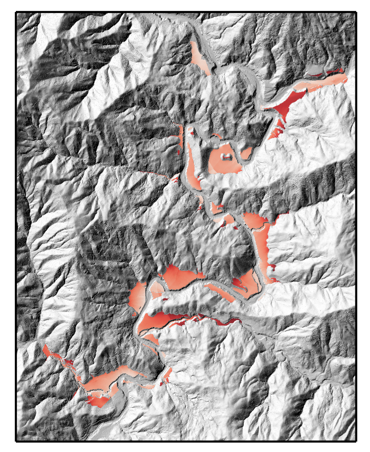
15. Calculating drainage density
Drainage density is a fundamental landscape metric which describes the total length of channels in a basin normalised by the basin area, first described by Horton (1945). In this chapter we describe how to calculate the drainage density and mean hilltop curvature of a specified order of drainage basins (for example, all second order basins). We also include code which will calculate the drainage density of each basin given a list of cosmogenic radionuclide (CRN)-derived erosion rate data. We used this code to examine the relationship between drainage density and erosion rate in our paper published in JGR Earth Surface in 2016.
Citation: Clubb, F. J., S. M. Mudd, M. Attal, D. T. Milodowski, and S. W. D. Grieve (2016), The relationship between drainage density, erosion rate, and hilltop curvature: Implications for sediment transport processes, J. Geophys. Res. Earth Surf., 121, doi:10.1002/2015JF003747.
15.1. Get the code for drainage density analysis
The code for the drainage density analysis can be found in our GitHub repository. This repository contains code for extracting the drainage density for a series of basins defined by points from cosmogenic radionuclide samples, as well as the drainage density and mean hilltop curvature for basins of a specified order.
15.1.1. Clone the GitHub repository
First navigate to the folder where you will keep the GitHub repository. If you have downloaded LSDTopoTools using vagrant, then this should be in the folder Git_projects. Please refer to the chapter on Installing LSDTopoTools using VirtualBox and Vagrant for more information on this. To navigate to this folder in a UNIX terminal use the cd command:
vagrant@vagrant-ubuntu-precise-32:/$ cd /LSDTopoTools
vagrant@vagrant-ubuntu-precise-32:/$ cd /Git_projects
You can use the command pwd to check you are in the right folder. Once you are in this folder, you can clone the repository from the GitHub website:
vagrant@vagrant-ubuntu-precise-32:/LSDTopoTools/Git_projects$ pwd
/LSDTopoTools/Git_projects
vagrant@vagrant-ubuntu-precise-32:/LSDTopoTools/Git_projects$ git clone https://github.com/LSDtopotools/LSDTopoTools_DrainageDensity.git
Navigate to this folder again using the cd command:
$ cd LSDTopoTools_DrainageDensity/15.1.2. Alternatively, get the zipped code
If you don’t want to use git, you can download a zipped version of the code:
vagrant@vagrant-ubuntu-precise-32:/LSDTopoTools/Git_projects$ pwd
/LSDTopoTools/Git_projects
vagrant@vagrant-ubuntu-precise-32:/LSDTopoTools/Git_projects$ wget https://github.com/LSDtopotools/LSDTopoTools_DrainageDensity/archive/master.zip
vagrant@vagrant-ubuntu-precise-32:/LSDTopoTools/Git_projects$ gunzip master.zip
GitHub zips all repositories into a file called master.zip,
so if you previously downloaded a zipper repository this will overwrite it.
|
15.1.3. Get the example datasets
We have provided some example datasets which you can use in order to test the drainage density analysis. In this tutorial we will work using a LiDAR dataset from the Guadalupe Mountains, New Mexico. This is a clip of the original dataset, which we have resampled to 2 m resolution. The full dataset is available from OpenTopography.. If you are using the vagrant distribution, create a new folder within the Topographic_projects folder, and then navigate to this folder:
vagrant@vagrant-ubuntu-precise-32:/LSDTopoTools/Topographic_projects$ mkdir Guadalupe_NM
vagrant@vagrant-ubuntu-precise-32:/LSDTopoTools/Topographic_projects$ cd Guadalupe_NM/
You can get the clip from our ExampleTopoDatasets repository using wget:
$ wget https://github.com/LSDtopotools/ExampleTopoDatasets/raw/master/Guadalupe_DEM.bil
$ wget https://github.com/LSDtopotools/ExampleTopoDatasets/raw/master/Guadalupe_DEM.hdr
This dataset is already in the preferred format for use with LSDTopoTools (the ENVI bil format). The figure below shows a shaded relief map of part of the Guadalupe Mountains DEM which will be used in these examples.
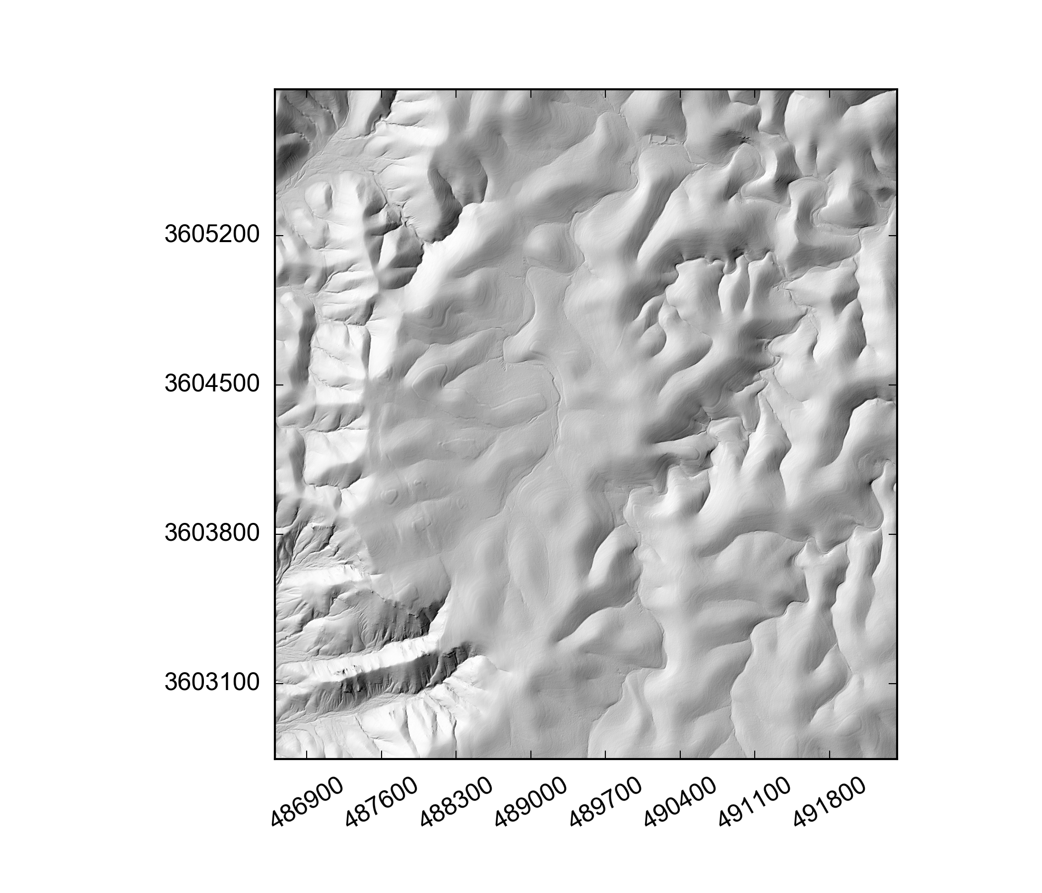
15.1.4. Get the example parameter files
We have also provided some examples parameter files that are used to run the drainage density analysis. These should be placed in the same folder as your DEM (e.g. in the folder /LSDTopoTools/Topographic_projects/Guadalupe_NM/. You can get the example parameter file using wget:
$ wget https://github.com/LSDtopotools/ExampleTopoDatasets/tree/master/example_parameter_files/drainage_density_guadalupe.driver15.1.5. Python scripts
We have also provided some Python scripts for creating figures from the draiange density analysis. These should produce similar figures to those in Clubb et al. (2016), JGR-ES. These scripts are in the directory Python_scripts within LSDTopoTools_DrainageDensity:
vagrant@vagrant-ubuntu-precise-32:/LSDTopoTools/Git_projects/LSDTopoTools_DrainageDensity$ cd Python_scripts
vagrant@vagrant-ubuntu-precise-32:/LSDTopoTools/Git_projects/LSDTopoTools_DrainageDensity/Python_scripts$ ls
drainage_density_plot.py	drainage_density_plot_cosmo.py
15.2. Preliminary steps
15.2.1. Getting the channel head file
Before the drainage density analysis can be run, you must create a channel network for your DEM. This can be done using the Channel extraction algorithms within LSDTopoTools. There are several channel extraction algorithms which you can choose from: for more details please refer to the Channel extraction section. Once you have run the channel extraction algorithm, you must make sure that the bil and hdr files with the channel head locations are placed in the same folder as the DEM you intend to use for the drainage density analysis.
15.2.2. Selecting a window size
Before we can run the drainage density algorithm, we need to calculate the correct window size for calculating mean hilltop curvature across the DEM. Please refer to the Selecting A Window Size section for information on how to calculate a window size for your DEM.
15.3. Analysing drainage density for all basins
This section provides instructions for how to extract the drainage density and mean hilltop curvature for every basin in the landscape of a given order (e.g. all second order drainage basins).
15.3.1. Creating the paramter file
In order to run the drainage density analysis code you must first create a parameter file for your DEM. This should be placed in the same folder as your DEM and the channel heads bil file. If you followed the instructions in the Get the code for drainage density analysis section then you will already have an example parameter file for the Guadalupe Mountains DEM called drainage_density_guadalupe.driver. Parameter files should have the following structure:
Name of the DEM without extension
Name of the channel heads file - will vary depending on your channel extraction method
Minimum slope for filling the DEM
Order of basins to extract
Window size (m): calculate for your DEM resolution
An example parameter file for the Guadalupe Mountains DEM is set out below:
Guadalupe_DEM
Guadalupe_DEM_CH_DrEICH
0.0001
2
6
15.3.2. Step 1: Get the junctions of all the basins
The first step of the analysis creates a text file with all the junction numbers of the basins of the specified stream order. Before the code can be run, you must compile it using the makefile in the folder LSDTopoTools_DrainageDensity/driver_functions_DrainageDensity. Navigate to the folder using the command:
$ cd driver_functions_DrainageDensity/and compile the code with:
$ make -f drainage_density_step1_junctions.makeThis may come up with some warnings, but should create the file drainage_density_step1_junctions.out. You can then run the program with:
$ ./drainage_density_step1_junctions.out /path/to/DEM/location/ name_of_parameter_file.driverFor our example, the command would be:
$ ./drainage_density_step1_junctions.out /LSDTopoTools/Topographic_projects/Guadalupe_NM/ drainage_density_guadalupe.driverThe program will create a text file called DEM_name_DD_junctions.txt which will be ingested by step 2 of the analysis. It will also create some new rasters:
-
DEM_name_fill: the filled DEM
-
DEM_name_HS: a hillshade of the DEM
-
DEM_name_SO: the channel network
-
DEM_name_JI: the locations of all the tributary junctions
-
DEM_name_CHT: the curvature for all the hilltops in the DEM
15.3.3. Step 2: Get the drainage density of each basin
The second step of the analysis ingests the junctions text file created in step 1. For each junction it will extract the upstream drainage basin, and calculate the drainage density and mean hilltop curvature for the basin. This will be written to a text file which can be plotted up using our Python script.
First, compile the code with the makefile:
$ make -f drainage_density_step2_basins.makeThis may come up with some warnings, but should create the file drainage_density_step2_basins.out. You can then run the program with:
$ ./drainage_density_step2_basins.out /path/to/DEM/location/ name_of_parameter_file.driverFor our example, the command would be:
$ ./drainage_density_step2_basins.out /LSDTopoTools/Topographic_projects/Guadalupe_NM/ drainage_density_guadalupe.driverThis program will create 2 text files. The first one will be called DEM_name_drainage_density_cloud.txt and will have 3 rows:
-
Drainage density of the basin
-
Mean hilltop curvature of the basin
-
Drainage area of the basin
This text file represents the data for every basin in the DEM. The second text file will be called DEM_name_drainage_density_binned.txt, where the drainage density and hilltop curvature data has been binned with a bin width of 0.005 m-1. It has 6 rows:
-
Mean hilltop curvature for the bin
-
Standard deviation of curvature
-
Standard error of curvature
-
Drainage density for the bin
-
Standard deviation of drainage density
-
Standard error of drainage density
These text files are read by drainage_density_plot.py to create plots of the drainage density and mean hilltop curvature. The code also produces DEM_name_basins.bil, which is a raster with all the basins analysed.
15.3.4. Step 3: Plotting the data
Navigate to the folder Python_scripts within the LSDTopoTools_DrainageDensity repository. You should find the following files:
vagrant@vagrant-ubuntu-precise-32:/LSDTopoTools/Git_projects/LSDTopoTools_DrainageDensity/Python_scripts$ ls
drainage_density_plot.py	drainage_density_plot_cosmo.py
Open the file called drainage_density_plot_cosmo.py. We suggest doing this on your host machine rather than the virtual machine: for instructions about how to install Python on your host machine please see the section on Getting python running.
Open the file called drainage_density_plot.py. We suggest doing this on your host machine rather than the virtual machine: for instructions about how to install Python on your host machine please see the section on Getting python running.
If you want to run the script on the example dataset you can just run it without changing anything. The script will create the file Guadalupe_DEM_drainage_density_all_basins.png in the same folder as your DEM is stored in. If you want to run it on your own data, simply open the Python script in your favourite text editor. At the bottom of the file you need to change the DataDirectory (Line 165) and the DEM identifier (Line 167) to reflect your data:
# Set the data directory here - this should point to the folder with your DEM
DataDirectory = 'C:\\vagrantboxes\\LSDTopoTools\\Topographic_projects\\Guadalupe_NM\\'
# Name of the DEM WITHOUT FILE EXTENSION
DEM_name = 'Guadalupe_DEM'
make_plots(DataDirectory, DEM_name)
You should end up with a plot like the one below:
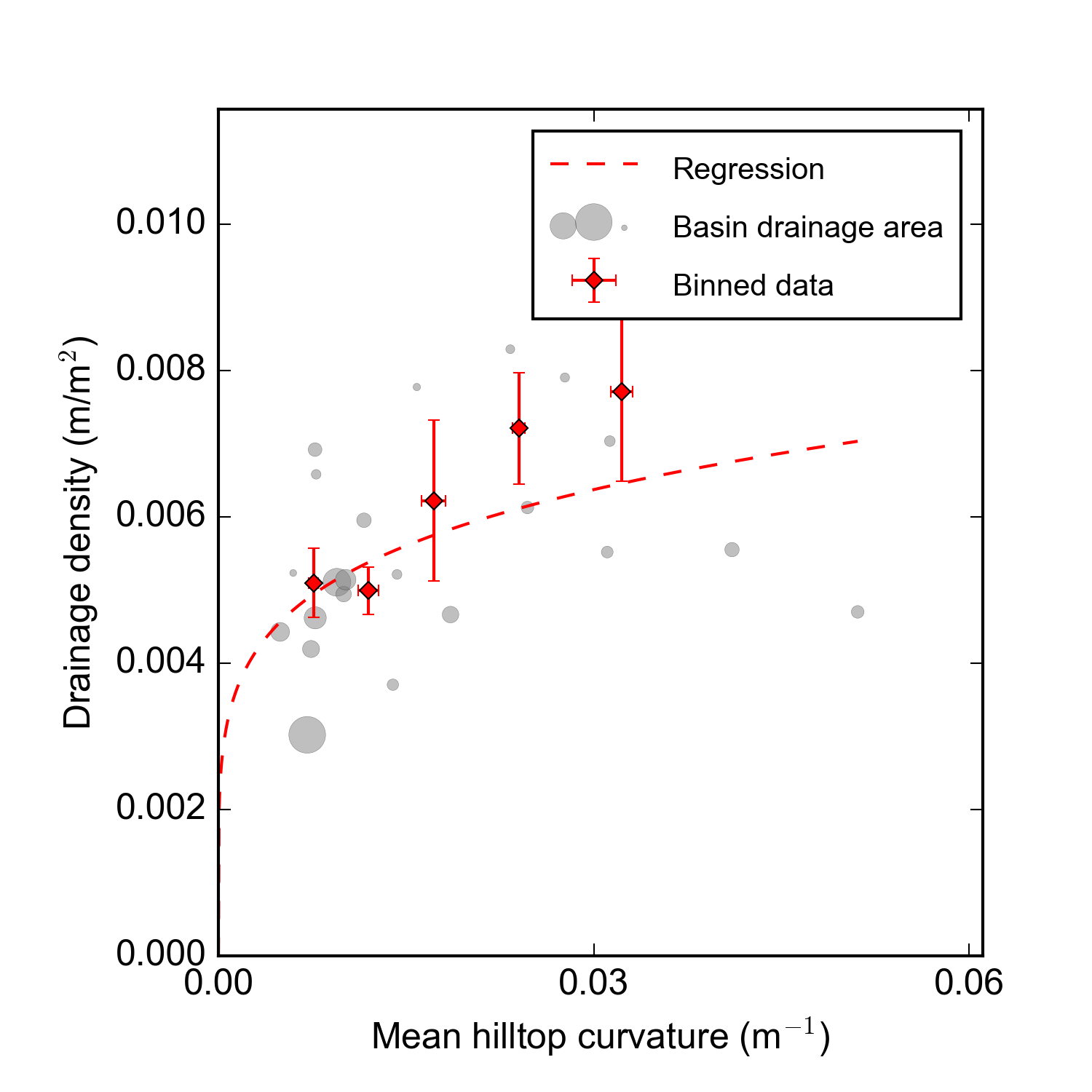
15.3.5. Summary
You should now be able to extract the drainage density and mean hilltop curvature for all basins of a given order for your DEM, and use Python to plot the results.
15.4. Analysing drainage density for basins with CRN-derived erosion rates
This section provides instructions for how to extract the drainage density for basins upstream of a series of point locations, such as cosmogenic radionuclide (CRN)-derived erosion rate samples. As an example, we will use the erosion rate data collected by Hurst et al. (2012) and Riebe et al. (2000) for the Feather River, Northern California. The lidar data for this area is available from OpenTopography. We haven’t included it in our example datasets as it is too large, but information on how to convert it into the right format can be found in our section on GDAL.
15.4.1. Formatting your erosion rate data
The program needs to read in a text file with the erosion rate data. This file needs to be called DEM_name_cosmo.txt where DEM_name is the name of the DEM without extension. The file should have a row for each sample, with 4 columns, each separated by a space:
-
X coordinate - same as DEM coordinate system
-
Y coordinate - same as DEM coordinate system
-
Erosion rate of the sample
-
Error of the sample
An example of the file for the Feather River is shown below (UTM Zone 10N):
640504.269	4391321.669	125.9	23.2
647490.779	4388656.033	253.8	66.6
648350.747	4388752.059	133.3	31.9
643053.985	4388961.321	25.2	2.7
643117.485	4389018.471	18.5	2
...
This file has to be stored in the same folder as your DEM.
15.4.2. Creating the paramter file
Along with the text file with the erosion rate data, you must also create a parameter file to run the code with. This should have the same format as the parameter file for running the analysis on all the basins, minus the last two lines. The format is shown below:
Name of the DEM without extension
Name of the channel heads file - will vary depending on your channel extraction method
Minimum slope for filling the DEM
This should also be stored in the same folder as your DEM.
15.4.3. Step 1: Run the code
Before the code can be run, you must compile it using the makefile in the folder LSDTopoTools_DrainageDensity/driver_functions_DrainageDensity. Navigate to the folder using the command:
$ cd driver_functions_DrainageDensity/and compile the code with:
$ make -f get_drainage_density_cosmo.makeThis may come up with some warnings, but should create the file get_drainage_density_cosmo.out. You can then run the program with:
$ ./get_drainage_density_cosmo.out /path/to/DEM/location/ name_of_parameter_file.driverwhere /path/to/DEM/location is the path to your DEM, and name_of_parameter_file.driver is the name of the parameter file you created.
The program will create a text file called DEM_name_drainage_density_cosmo.txt which can be ingested by our Python script to plot up the data. This file has 9 rows with the following data:
-
Drainage density of the basin
-
Mean basin slope
-
Standard deviation of slope
-
Standard error of slope
-
Basin erosion rate
-
Error of the basin erosion rate
-
Basin drainage area
-
Mean hilltop curvature of the basin
-
Standard error of hilltop curavture
It will also create some new rasters:
-
DEM_name_slope: slope of the DEM
-
DEM_name_curv: curvature of the DEM
15.4.4. Step 2: Plot the data
Navigate to the folder Python_scripts within the LSDTopoTools_DrainageDensity repository. You should find the following files:
vagrant@vagrant-ubuntu-precise-32:/LSDTopoTools/Git_projects/LSDTopoTools_DrainageDensity/Python_scripts$ ls
drainage_density_plot.py	drainage_density_plot_cosmo.py
Open the file called drainage_density_plot_cosmo.py. We suggest doing this on your host machine rather than the virtual machine: for instructions about how to install Python on your host machine please see the section on Getting python running.
Open the Python script in your favourite text editor. At the bottom of the file you need to change the DataDirectory (Line 131) and the DEM identifier (Line 133) to reflect your data:
# change this to the path to your DEM
DataDirectory = 'C:\\vagrantboxes\\LSDTopoTools\\Topographic_projects\\Feather_River\\'
# Name of the DEM WITHOUT FILE EXTENSION
DEM_name = 'fr1m_nogaps'
make_plots(DataDirectory, DEM_name)
You should end up with a plot like the one below:
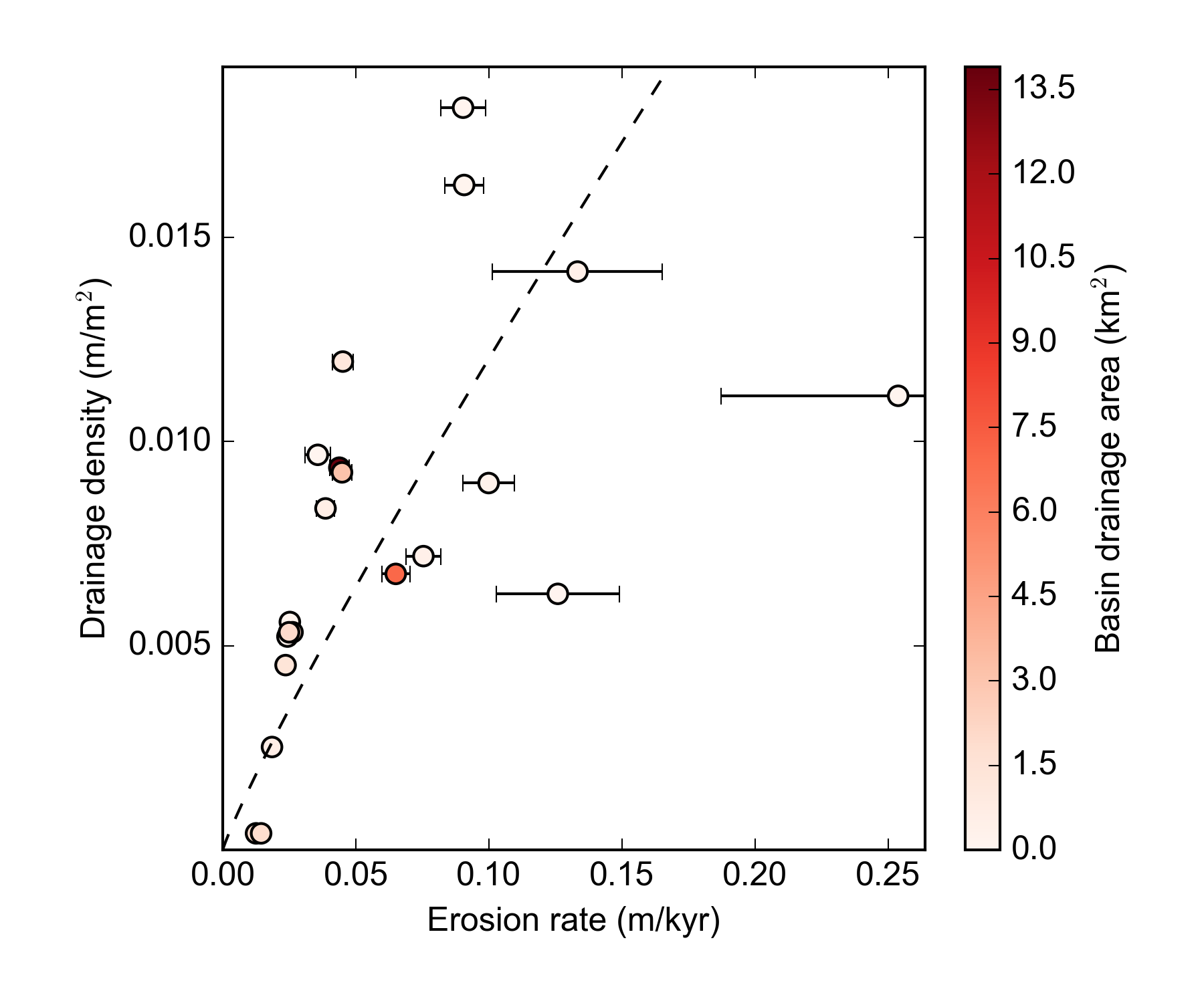
15.4.5. Summary
You should now be able to extract the drainage density for a series of different basins across the landscape. These can either be all basins of a specific order (Step 1), or basins defined by point coordinates (e.g. for catchment-averaged erosion rates from CRN samples in Step 2).
16. Hydrological and Erosion Modelling
| LSDCatchmentModel is a 2.5D 'hydrodynamic' landscape evolution model that simulates flooding and erosional processes at the catchment scale, on the order of hours to 100s of years. |
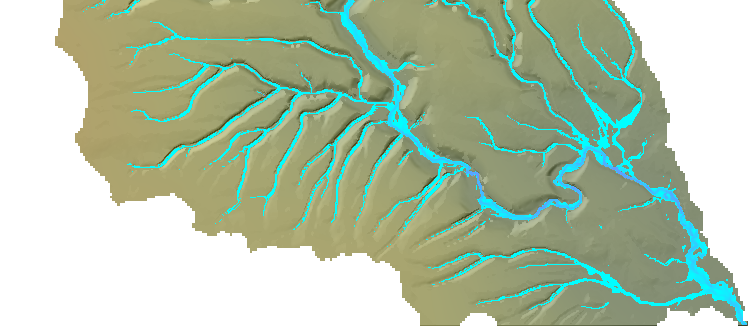
Numerical models are useful tools for testing hypotheses of geomorphic processes and landscape evolution. Long term landscape evolution takes place over extensive geological time periods, but is controlled by the dynamics of water flow, and sediment transport within river catchments on much shorter, day-to-day time scales. The LSDTopoTools package provides a model for simulating catchment processes at short-term scales, with the LSDCatchmentModel package.
This chapter documents how to use the LSDCatchmentModel to set up and run simulations of hydrology and catchment-scale erosion and evolution. LSDCatchmentModel is a 2.5D numerical model of landscape evolution based on the CAESAR-Lisflood model (Coulthard et al., 2013). The model is a Cellular Automaton model, whereby the grid cells in the model domain each have their own parameters associated with them (such as elevation, water depth, water velocity, sediment load, etc.) and the change in these parameters is determined by the state of the neighbouring grid cells.
Unlike many models of landscape evolution, this model features an explicit calculation of water flow through the landscape based on a highly simplified form of the shallow water equations (Bates et al., 2010). Most other models, in order to simulate long term evolution, rely on approximations for water discharge based on drainage area, and assume instantaneous run-off of water under hydrological steady-state conditions. The LSDCatchmentModel is therefore suited to modelling both flooding and erosional processes. It can be run as a standalone hydrological model (no erosion) if so desired.
The model is also developed to run on parallel computing architectures (Multi-core/cluster computers).
16.1. Origins: relation to CAESAR-Lisflood
The model is based on a 'light', stripped-down C++ translation of the CAESAR-Lisflood model. Unlike the CAESAR model, there is no graphical user interface (GUI), as in keeping with the LSDTopoTools mantra, the code is designed to be run from a command line, console, or terminal interace. This helps facilitate geomorphic modelling that is not dependent on a series of mouse-clicks, or propriatary operating systems and libraries. The Catchment Model code can be run on a range of operating systems and computing platforms, including Linux, MacOS, and Windows. However, GUIs can be useful for modelling, so if you would prefer to use a model in GUI-mode then CAESAR-Lisflood is a good choice for this. The LSDCatchmentModel model is designed to reproduce some of the core functionality in CAESAR-Lisflood, while being faster and cross platform, and to scale up to running on a supercomputer if the resources are available to you. One of the limitations for some users of CAESAR-Lisflood is that you need a dedicated Windows box to do your simulations, and you can’t send them off to a cluster computer-type facility, which typically run Unix-based operating systems. (Unless you have a bunch of spare Windows PCs…)
With the LSDTopoTools implementation you can also perform topographic analysis within the same software environment, switching easily between modelling and topographic analysis outputs.
| There is no current plan to maintain the code in tandem with CAESAR-Lisflood. LSDCatchmentModel was spun-off at CL v1.8f. |
16.2. Compilation
Several versions of the make file are provided, for different situations. It is planned in the future to make a single proper makefile with different options that cover the separate versions at present. For now, you will have to select from one of the following:
-
CatchmentModel_GCC_DEBUG.make
-
CatchmentModel_GCC_Optimised.make
The debug makefile (Option 1) contains all the compiler flags for debugging and profiling. (The program will run slower if you use this version - only use it for development or if trying to trace a bug). The optimised version (Option 2) runs with the -O2 flags and no profiler or debugger information. Both versions are set up for running the code in parallel on multiple cores. This applies to desktop PCs with multiple cores as well as compiling for single compute nodes on supercomputers (cluster computers).
Should you not have the OpenMP librares installed, or you wish to compile in serial mode (run on a single core/thread), remove the -fopenmp flags from the makefile, as well as the -DOMP_COMPILE_FOR_PARALLEL flag.
To compile, run make as follows with the makefile of your choice:
make -f CatchmentModel_GCC_Optimised.makeIf you want to start again and remove the object and executable files, there is also a clean command:
make -f CatchmentModel_GCC_Optimised.make cleanYou will get an executable called CatchmentModel_OpenMP_Optimised.out or similar, depending on which makefile you used.
16.2.1. Dependencies
| Your compiler must support C++11. Almost all compilers do as of 2016, as long as you are running a fairly recent version. (GCC version 4.7 onwards should be fine, preferrably GCC 4.8+) Currently, support is not usually enabled by default. (UPDATE 2016: It is in GCC 6.1) The C++11 flag to turn it on is included in the makefile. The code uses some features of the C++11 language standard not supported by older standards. You don’t need to know any about it at this stage. |
The parallel version of the code uses the OpenMP libraries, which are powerful (and somewhat magical…) libraries for compiling the code to run in parallel. These are widely supported libraries and many systems will come with them pre-installed. But you may need to install the gcc-devel package on linux, if using gcc. Again, the compiler flag is taken care of in the makefile. The code has been tested on the gcc (versions 4.8 and above) Cray compiler, and icc (Intel) compiler v12.
All other libraries are supplied with the source code (The TNT, Template Numerical Toolkit library, which provides array/matrix structures for the model data). You do not need to install them separately.
16.3. Running the Model
The model runs from the command line/terminal/console. You specify the model executable name (CatchmentModel.out) followed by the path name to the parameter file and the parameter file itself. The model will print out updates to the terminal window regularly, keeping you updated to the stage it is at and if there are any errors. The DEM of your catchment must be present in the same folder as your parameter file and must be correctly formatted.
You need a minimum of three input files:
-
Parameter file
-
DEM file of your catchment (currently only ASCII format is supported, sorry
.bil/fltfans!) -
Rainfall time series text file (There is currently no option to generate rainfall within the model, but this is coming soon)
Your input files (DEM etc, parameter file) can be in any folder you like, as the path to the input files is specified in the parameter file. This means the executable file can be kept separate, once it has been compiled.
The model is run like so:
./CatchmentModel.out [PATH-TO-FOLDER-WITH-INPUT-FILES] ParameterFile.txtAs you can see, the executable takes two arguments, the first is the path where your parameter file and input files can be found, the second is the name of your parameter file. Note that the names of the input DEM and rainfall file are specified in the parameter file.
When the model runs, it will print to screen the parameters that have been read from the parameter file, for a sanity check. The debug version prints a lot of other information to screen, to help find bugs and errors. I suggest turning this off and running with the optimised version unless you are trying to trace a bug. The program will update you at certain stages of the data ingestion process. (This usually only takes a few seconds). When the model runs, a counter displays the number of elapsed minutes in model-time. (There is an option to turn this off in the parameter file - set debug_print_cycle_on to no.
The model also prints out when it is writing output raster files, such as water depths, elevation difference etc. These files are outputted to the directory specified in the parameter file.
16.3.1. Outputs
CatchmentModel generates similar outputs to CAESAR-Lisflood, i.e. a timeseries text file of the water discharge, and sediment fluxes; as well as raster files for water depths, elevations, erosion amounts, and so on. These can be outputted at an interval specified in the parameter file. Output files can be saved in ascii (.asc), or binary (.flt) format.
16.3.2. DEM preparation
| You will need to check your DEM is correctly formatted before use. LSDCatchmentModel has specific requirements about DEM layout. |
Currently, you will have to prepare your own DEM as a separate stage in the workflow. (Using whichever GIS tool you like, or preferably our own software!). The DEM should be set up so that one side of the catchment will act as the flow exit point. If you do not have the intended catchment outlet point touching one of the DEM edges, you will get unrealistic pooling of water and flood the entire catchment, as water will not be able to leave the model domain. In other words: There should be no 'NODATA' values between the intended outlet cell(s) and the edge the DEM file. This is very important for the model to work correctly. You may have to rotate your DEM or add on a channel artificially so that your catchment has a suitable outlet point at one side of the DEM file.
| The model will actually route water off all edges of the catchment, if the geometry of your catchment allows it. This might be fine for your intended use, but note that the discharge timeseries file will report total water discharge and sediment output as a total from ALL edge cells, not just the ones you think are the main catchment outlet point. As a side effect, you can use the model to simulate range scale runoff and multiple catchments, just be aware that you will get one value for total discharge for the whole DEM. |
Technically, the DEM doesn’t need to be pit-filled, but it may be worthwhile to do so as parts of the model can be sped up when the catchment is in a low-flow or steady-flow state. Again, it depends on your intended usage of the model.
16.3.3. Model run time controls
A sample parameter file is provided for the Boscastle floods simulation. This is a 48-hour simulation using a 5m DEM, over a catchment 3km x 5.5km (about 700000 grid cells). It will take about 2-3 hours to run on a mid-range Desktop machine. (You can dramatically speed this up by using a coarser DEM.) Number of domain grid cells is the main control on compute time. With a multi-core machine, the run time can be significantly reduced, depending on the number of cores you have.
| If using the OpenMP makefile, you can get this down to around 11 minutes using a 48-core machine. Use it if you have the hardware! |
Note that some of the parameters in the paramter file will have an effect on model run time. For example: in_out_difference, courant_number, and many of the minimum threshold values for flow and erosion can all be tweaked to get model speed up in some way. See the parameter file guide for advice.
16.4. Parameter File
The parameter file is read by the CatchmentModel program when it starts, setting the variables for various components of the model, as well as the names of the DEM files and supplementary input files needed for the model simulation. It is a plain text file and can be called anything you like. By convention, the example parameter file supplied with the code has the suffix .params, but you may use whatever you like.
Anything in the parameter file preceded by a # will be treated as a comment. You are free to comment away in the parameter file to your heart’s content.
The order of the parameters in the parameter file is not strict, but we stick to the convention used in the sample file for reference here. The parameter names must not be changed, and must be lowercase.
| Parameter Name | Units/Data Type | Description | ||
|---|---|---|---|---|
|
text |
The name of your DEM that will act as the terrain surface in the model. Do not give the extension here. |
||
|
text |
The extension of the input DEM. Only ASCII (asc) is currently supported, we are working on supporting other input formats soon. |
||
|
text |
The format to save output rasters in. Supported choices are: 'asc' or 'flt' (binary). 'bil' also works but no georeferencing is supported yet. |
||
|
text |
The path where your input files can be found |
||
|
text |
The path where your output files will be written |
||
|
text |
A name for the output timeseries file. You can supply your own extension, but it will always be a plain text file. |
||
|
model minutes/integer |
Will record a timeseries record (new row) every X minutes in model time. The timeseries output contains the discharge of water and sediment. |
||
|
||||
|
text |
The hydroindex file name (with extension). Only ascii (asc) currently supported. |
||
|
text |
The rainfall data file name (with extension). Must be a plain text file. |
||
|
text |
Name of your grain data input file. |
||
|
text |
Name of the bedrock DEM. If specified, this DEM (ascii only) will be loaded as a solid bedrock layer beneath your top-layer terrain DEM. It’s up to the use to make sure the elevations are lower than the top layer! |
||
|
||||
|
model seconds, integer |
The minimum timestep used in the model |
||
|
model seconds, integer |
Maximum timestep used by model. Should not really be higher than your rainfall data interval, otherwise you will skip input data. |
||
|
model hours, integer |
Length of your simulation, minus 1. (So for a 72 hour simulation, enter '71' here.) This is a weird quirk that will be fixed in a later release. |
||
|
Ignore, leave at 1. |
|||
|
||||
|
text |
Can either be wilcock or einstein. Determines which sediment transport law is used by the model. |
||
|
meters/second |
Limits the maximum velocity used to calculate sediment transport. The default is 5. It is rarely invoked except in very steep slopes. |
||
|
metres |
This controls the thickness of layer representing the surface, bedload or subsurface. It should be around 0.1 to 0.2. It must be at least 4 times the erode_limit parameter. (See below) |
||
|
In channel lateral erosion rate. Prevents overdeepening feedback. See explanation here |
|||
|
metres |
Maximum erosion limit per cell (or deposition). Prevents numerical instabilities by transferring too much between cell to cell. Should be around 0.01 for 10m or less DEMs, slightly higher for coarse DEMs. |
||
|
boolean (yes/no) |
Turns on suspended sediment for the first fraction only at present. |
||
|
boolean (yes/no) |
Reads in the initial grain size data from a file. Normally the initial distribution of grainsizes is uniform across the landscape if this is not specified. |
||
|
||||
|
boolean (yes/no) |
Turns on lateral erosion in channels (UNTESTED) |
||
|
See Coulthard and Van de Wiel (2007) for details. This parameter sets the lateral erosion rates, and ought to be calibrated to a field site. Values can ramge from 0.01-0.001 for braided rivers; 0.0001 for meandering channels. This value is grid cell size independent. |
|||
|
integer |
Determines how well smoothed the curvature of the channels will be. Should be set as the frequency of meanders/distance between two meanders in grid cell size. |
||
|
integer |
The gradient used to determine lateral erosion rates can be shifted downstream, allowing meander bars and bends to migrate down channel. Suggested values are around 10% of the edge_smoothing_passes parameter. So around 1-5. |
||
|
The maximum difference allowed in the the cross channel smoothing of edge values. After calculating the radius of curvature for the outside of a meander bend, the model must interpolate this value to determine how much sediment can be moved laterally. Smaller values result in better cross channel gradients, but take up more CPU time. Typical default value is 0.0001. If your channels are well resolved by DEM resolution, you may need to reduce by an order of magnitude. |
|||
|
||||
|
boolean (yes/no) |
Runs the model as a hydrological/flood inundation model only if set to yes. Will turn off all the erosion routines and terrain will be fixed. Speeds up run times considerably. |
||
|
As well as the water routing sub-model, LSDCatchmentModel also calculates the discharge based on Beven’s TOPMODEL (i.e. discharge approximation based on drainage area and topography. The model contains the infamous m parameter, which varies depending on environment. You should consult the literature for appropriate values.
|
|||
|
cumecs |
If greater than 0, allows the model to run faster in periods of hydrological steady state. If the difference between water entering the catchment and water leaving the catchment is equal to or less than this value, the model will increase the time step. The time step will then be determined by erosional and depositional processes, which are typically much slower acting. Can be set to a low mean annual flow value for the river. |
||
|
cumecs |
Threshold for calculating flow depths. The model will not calculate flow depths when the discharge at a cell is below this value, avoiding CPU time spent calculating incredibly small flow amounts. Should be set to approximately 10% of grid cell size. e.g 0.5 for a 50m DEM. |
||
|
cumecs |
An upper discharge threshold that will prevent water being added above the given discharge threshold. Typically 1000.0, but lowering the value will shift the balance of water being added to the headwaters, rather than lower down through the catchment. |
||
|
metres |
If water depths are below this threshold, the model will not calculate erosion for that cell in that timestep. Used to prevent CPU time being spent on incredibly small amounts of erosion calculations. |
||
|
The slope used to calculate water flow on the edge of the DEM (since there is no neighbouring cell to calculate the downstream gradient. You should set this to approximately the same as the average channel gradient near the outlet of your river. |
|||
|
Untested/unimplemented yet |
|||
|
Controls the numerical stability and execution speed of the flow model. See Bates et al (2009). Typical values should be between 0.3 and 0.7. Higher values will speed up the model, but are more unstable. Parameter is dependent on grid cell size. DEMs of 20-50m resolution can use values of 0.7, finer DEMs (e.g. <2m) will need the lowest value of 0.3, but do not set it lower than 0.3. |
|||
|
Restricts flow between cells per time step, as too much can lead to checkerboarding effects. If this happens the froude number can be lowered. The default value of 0.8 results in subcritical flow - flow dominated by gravitational forces and behving in a slow or stable way. A value of 1 results in critical flow, which may be ok for shallow flows at coarse grid cell resolutions. Note that reducing flow with the Froude number will reduce the speed of a flood wave moving downstream. |
|||
|
A roughness coefficient used by the flow model. Values can be looked-up here. |
|||
|
metres |
This threshold prevents water being routed between adjacent cells when the gradient is incredibly small. A good default value is 0.00001. |
||
16.5. Running the code in Parallel
I’ve mentioned that the code has features that allow certain sections to run on parallel computing technology, such as a multi-core desktop PC, or a cluster computer with multiple CPUs. The included makefiles will compile this feature by deafult, and most computers are set up to run in parallel, given appropriate software. However, it is a good idea to double check your computing environment is set up correctly for parallel execution of the code.
On linux, commands such as nproc will tell you how many CPUs/cores you have availble. (A decent desktop PC might have 4-8 cores, for example). On linux, you can set the number of execution threads to match the number of cores by doing:
export OMP_NUM_THREADS=X
where X is the number of threads (set it to the same number of cores available for best performance.) So for an 8 core machine, set this value to 8. Some environments will already have this set up automatically, but I do it just to be sure my code will use all the availble cores.
16.6. Notes for HPC use
As it currently stands, CatchmentModel is designed for shared-memory architectures, i.e. single-nodes on cluster machines. Of course, you can take advantage of HPC services, as they usually high-spec compute nodes with decent numbers of CPUs and memory. The code lends itself well to 'embarassingly' parallel task farming, whereby you run multiple instances of the code with different datasets or parameters, for example. An HPC service is very useful for this as you can set potentially hundreds of simulations going at the same time, and get your results back much quicker. Consult your friendly HPC service for details of how to do this, as the instructions will vary between HPC environment.
17. Landscape Evolution Modelling with LSDTopoTools
The LSD Topo Toolbox contains a landscape evolution model. The model implementation is contained in the LSDRasterModel files. The driver file is model_driver.cpp. The landscape model is partly based on the FastScape algorithm (Braun 2013), an efficient method for solving the stream power law for fluvial incision, as well as the MUDDPile algorithms for hillslope evolution. It contains both hillslope and fluvial components, which can be run individually, simulating a single hillside for example, or together, to simulate whole landscape evolution. The model will run from default parameters if none are supplied, but the user can also specify their own choice of parameters for the model run, which are detailed below.
17.1. Model Parameters and Components
17.1.1. Model Domain
This is the name that will be appened to all output files generated during the model run. The model will check to see if this name has already been used before overwriting existing output files.
This is the number of rows in the model domain. You can also think of it as the y dimension of the model grid.
This is the number of columns in the model domain. You can also think of it as thee x dimension of the model grid.
The resolution of the model grid. The size in metres that a single grid cell represents.
Boundary code This code determines the output sides of the model grid. I.e. which sides are for sediment output and which are not. The b represents base level, n represents no flow, and p represents periodic boundary conditions.
The model timestep, dt
The end time for the model run
This sets the model to either run until it reaches steady state (=1), or until a specified time (=0).
Instructs the model to use block, uniform uplift, or an uplift field.
The uplift rate (m/yr)
This parameter sets the iteration tolerance value in the LSDRasterModel object. The value is related to the implicit solver and when the solution is considered to be 'converged upon' and the numerical soultion solved. (DAV - needs more explanation?)
The output file interval.
17.1.2. Fluvial Component
Turns the fluvial component on or off, with these respective keywords.
The K paramter used in the many forms of the stream power equation and its derivatives. K can also be thought of as the erodibility. Typical values for K are something like 0.0001 to 0.002, but these can vary significantly between different lithologies/environments etc. The default is 0.0002.
The m exponent of the stream power law. Typical values of the m/n ratio are between 0.3 and 0.7, but consult the literature if it is availble for your study area. The ratio is related to the concavity of the idealised river profile. The default value of m is 0.5.
The n exponent of the stream power law. Typical values are around 1.0. (Which is the default value). The above parameters are related to each other in the stream power equation as below:
\(I = KA^mS^n\)
where I is the incision rate, A is the drainage area, and S is the slope of the channel. The fluvial component of the model is based on this equation, which is a good approximation in many bedrock mountainous landscapes, though your mileage may vary.
Sets the K value to be constant (0 is default, meaning constant).
17.1.3. Hillslope Component
The hillslope component comes in two flavours, a linear model and a non-linear one.
Turns the hillslope component on or off
Sets the hillslope law to linear or non-linear. (on or off)
The soil transport coefficient. The D value is used in calculating the soil creep functions in the model.
The critical slope angle. The default is 30 degrees.
17.2. Running the Model
Once compiled, the model is run using:
./model.out [parameter.file] [run_name]Screen output should help the user see if the components/parameters have run as expected.
17.3. Model Output
Appendix A: Software
There are quite a few different components you need to get working on your system to perform the examples in this book (sorry!). Some of these are essential, and some are optional and included for completeness. In the following appendices, instructions for getting them installed on Windows or Linux are included. Since the author of this book does not have any computers running on friut-based operating system, I’m afraid instructions for getting the software working on such systems will require a bit of homework, but in theory installation on such systems should be similar to installation on Linux systems.
A.1. Essentials
The following tools are core to the contents of this book, and will need to be installed before you can work on the exercises in the book.
A.1.1. Git
Git is version control software. It helps you keep track of changes to your scripts, notes, papers, etc. It also facilitates communication and collaboration through the online communities github and bitbucket. The source code for LSDTopoTools is on github so by using Git you can make sure you always have the latest version of the software.
A.1.2. C++ tools
A number of scientific programs are written in these languages so information on how to get them working on your windows machine is incluided here for completeness.
To get these working you will need
-
The compiler. This is what translates the program into something the computer can understand.
-
The tool
make, which automates building programs. -
The tool
gdb. which stands for gnu debugger, a tool for debugging code. -
The tool
gprof, which is a profiler: it allows you to see which parts of your code are using the most computational resources.
A.1.3. Python
Python is a programming language used by many scientists to visualize data and crunch numbers. You can also use it to automate data management.
You will need:
-
The python programming language
-
Scipy, for scientific python. It includes lots of useful packages like
-
Numpy for fast numerics.
-
Matplotlib for plotting.
-
Pandas for data analysis.
-
-
pip for python package management.
-
A.1.4. GDAL
GDAL (the Geospatial Data Abstraction Library) is used to manipulate topographic data so that it can be fed into LSDTopoTools.
A.2. Useful extras
You could find these tools useful. In particular, my documentation is written using something called asciidoctor, which is implemented in a programming language called Ruby.
A.2.1. A virtual machine
This is essential if you are going to follow our instructions for Installing LSDTopoTools using VirtualBox and Vagrant, which is propbably what you will want to do if you do not have a Linux machine.
To do this you will need to intall Vagrant and VirtualBox.
A.2.2. Geographic Information Software
If you want to look at the data produced by LSDTopoTools, you could use our lightweight python tools, but in many cases you will want to use a GIS.
The common options are:
-
ArcGIS The GIS most frequently used by commercial enterprise and government. It is commercial software and rather expensive. If your organisation has a licence, fantastic. However not all users of our software will have a licence so all tutorials in this book will be based on open source software.
-
QGIS A GIS that behaves much like ArcGIS, but is open source.
-
Whitebox A very lightweight, open source GIS written in java. This is handy since it is quite portable: there is nothing to install, just copy the
.jarfile on your computer and away you go!
A.2.3. Ruby
Ruby is a programming language used frequently by web developers and has many package for building documentation and automating collection of data over the internet. In this book we will really only use it for documentation, but there is a large ecosystem of open source tools available in Ruby. It hasn’t been adopted to a great extent by the scientific community but you may still find useful tools, particularly if you are gathering online information.
The main reason we use Ruby is to generate our documentation using Asciidoctor, so if you fancy contributing to the documentation of getting the latest version, you will need to get Ruby and some associated tools.
You will need:
-
The Ruby programming language
-
Rubygems for updating ruby.
-
bumdler for managing updates and making sure scripts are up to date.
-
RubyDev kit which is needed for some other Ruby packages.
-
asciidoctor for making notes, documentation and books.
-
Ruby DevKit which is used by some Ruby extensions.
-
-
In addition you will need Node.js for some of the Ruby tools to work.
Appendix B: Using the LSDTopoToolsSetup.py script
To help you set up LSDTopoTools, we have written a series of modules in python that automate the creation of our standard directory structure, downloading of the source code and compiling the source code into programs. The script is called LSDTopoToolsSetup.py.
B.1. Getting the LSDTopoTools setup script
LSDTopoTools works in all popular operating systems (Windows, MacOS, Linux) by using Vagrant to create a Linux server within your host operating system: if you are not in a native Linux environment you should start a Vagrant server by following these directions.
Once you have done that, you should be able to ssh into a Linux session using putty.exe on Windows or the vagrant ssh command in MacOS and Linux.
Once you are in a Linux operating system, the easiest way to get the script is to use the utility wget:
$ wget https://raw.githubusercontent.com/LSDtopotools/LSDAutomation/master/LSDTopoToolsSetup.pyB.1.1. Alternatives to wget
You can also get the script by cloning the LSDAutomation repository:
$ git clone https://github.com/LSDtopotools/LSDAutomation.gitor you can got to the raw text of the file, then copy the text and paste into your favourite text editor (i.e. Brackets). You should save the file as LSDTopoToolsSetup.py.
B.2. Running the LSDTopoTools setup script
The setup script is a python script so you need python to run it. It should be run in Linux, so if you do not have a native Linux operating system the script should be run in your Vagrant server. Almost all flavours of Linux come with python installed as default (the Ubuntu system installed by our vagrantfiles is one example) so we will assume you have python.
The script requires parameters; if you run the script with no parameters, it will give you a message telling you what to do:
$ python LSDTopoToolsSetup.py

=======================================================================
Hello there, I am the going to help you set up LSDTopoTools!
You will need to tell me what to do.
If you are in vagrant, LSDTopoTools will always be installed in the root directory (\).
If you are not in vagrant,
LSDTopoTools will be installed in your home directory if you run this with:
   python LSDTopoToolsSetup.py -id 0

Or your current directory.
(i.e., the directory from which you called this program)

if you run with this:
   python LSDTopoToolsSetup.py -id 1

For help type:
   python LSDTopoToolsSetup.py -h

=======================================================================
B.2.1. Looking at all the LSDTopoToolsSetup options
You can call help for the LSDTopoToolsSetup.py script with:
$ python LSDTopoToolsSetup.py -hB.2.2. A default setup
In fact, there is no default setup, since you have to tell the tool where to install LSDTopoTools. You do this by using the -id flag.
-
If you select 0, LSDTopoTools will be installed in your home directory, which you can get to with the command
cd ~. -
If you select 1, LSDTopoTools will be installed in the current directory (i.e. the directory where the script is located).
-
If you are running a vagrant machine, these instructions will be ignored and LSDTopoTools will be installed in the root directory (you can get there with the command
cd \).
This will install a directory LSDTopoTools with subdirectories Git_projects and Topographic_projects. Each of these folders will clone subfolders from our github pages, and will compile the Analysis_driver as well as the chi_tool.
The directories will look like this:
/LSDTopoTools
  |--Git_projects
  |----LSDTopoTools_AnalysisDriver
  |----LSDTopoTools_ChiMudd2014
  |--Topographic_projects
  |----LSDTT_workshop_data
  |----Test_data
B.2.3. Other setup options
There are a number of other options on LSDTopoToolsSetup.py, which we will list here, as well as in the table below.
-
-CE TrueClone and compile the channel extraction programs used in Clubb et al, WRR, 2014. -
-MChi TrueClone and compile the tools for performing the chi analysis of Mudd et al., JGR-ES, 2014. -
-CRN TrueClone and compile the tools for calculating basinwide denudation rates from the cosmogenic nuclides 10Be and 26Al Mudd et al., ESURF, 2016. -
-cp TrueCheck the path names in all the subfolders inTopographic_projectsto reflect your own directory structure.
B.2.4. If you are running on native Linux
If your native operating system is Linux, you should be able to get LSDTopoTools working very quickly using LSDTopoToolsSetup.py without having to use vagrant. However, you do need to ensure that you have the utilities make, the gnu Pass:[C++] compiler installed, and also you need FFTW installed. If you are in Ubuntu installing FFTW is as easy as: sudo apt-get install -y libfftw3-dev. If you are in another flavour of Linux you will need to follow the full setup, which is described on the FFTW website. Once you have that stuff working, you can use LSDTopoToolsSetup.py to get everything working in a jiffy.
B.3. Table of LSDTopoToolsSetup.py options
| Flag | Input type | Description |
|---|---|---|
|
Integer, either 0 or 1 |
0 == home directory, 1 == current directory. If you are in vagrant it will ignore this option and install in the root directory. |
|
Boolean (either True or False) |
If this is True, installs the CAIRN CRN package for calculating basinwide denudation rates from the cosmogenic nuclides 10Be and 26Al Mudd et al., ESURF, 2016. |
|
Boolean (either True or False) |
If this is True, installs the channel extraction programs used in Clubb et al, WRR, 2014. |
|
Boolean (either True or False) |
If this is True, installs the tools for performing the chi analysis of Mudd et al., JGR-ES, 2014. |
|
Boolean (either True or False) |
If this is True, checks the pathnames of the parameter files |
Appendix C: Setting up on Windows
| You should only do this if you are some kind of Windows purist (does such a thing exist?). LSDTopoTools works best in Linux and at the moment the best way to get a linux server working within your Windows machine is to use Vagrant. Instructions can be found here: Installing LSDTopoTools using VirtualBox and Vagrant. |
For the kind of scientific tools we will be using, Windows can sometimes be a bit difficult, since many scientific developers work in Linux and so installation for their software is easiest in a Linux environment. However, you can get Windows to behave a bit like Linux which will make your life easier for the purposes of installing the required software for the examples here.
Alternatively, you can get a "virtual" Linux machine running on your Windows machine.
Let me type that in bold text: it will be far easier to do things in a Linux environment than in a Windows environment. I strongly encourage you to use our Vagrant setup.
C.1. Working with the powershell
Much of what we do will be through a powershell window. This is a text-based interface into your windows system that allows you to install software and run scripts and code. It functions like a linux terminal.
First of all, you need to get a powershell running. On my windows version, you just type powershell into the bit of Windows where you searh for files or programs (it varies based on what windows system you are using). You should be able to find a way to get a powershell on your version of windows through the power of the internet.
C.1.1. Starting a powershell session
First, you will need to open an administrator powershell. In your powershell window, type
PS> Start-Process powershell -Verb runAs
The PS> denotes the powershell propmpt.
|
| You might not have administrator priviliges on your computer. In that case you will need to convince the administrator to install everything for you, or you can ask them to install a linux virtual machine, which is described in the section Installing LSDTopoTools using VirtualBox and Vagrant. |
C.2. Windows installation programs
Take a deep breath. I am afraid this is going to take a while. You might consider following our instructions for Installing LSDTopoTools using VirtualBox and Vagrant instead of trying to get the software installed within a Windows environment.
| It is MUCH easier to run LSDTopoTools software in Vagrant server, but you should install programs for looking at your data (i.e., python, a GIS) on your host operating system (in this case Windows). |
C.2.1. A text editor
C.2.2. Git
Download and install git for windows.
There will be some options for you to select once you do this: the main one is something about line endings. I chose the "don’t change line endings" option.
Once this is installed you can right click on any folder in windows explorer and select the option git bash here. This will open a powershell window with git enabled. From there you can follow the instructions in the git chapter of this book.
C.2.3. Python on Windows with miniconda
The best way to install python is miniconda. We will use Python 2.7, so use the Python 2.7 installer.
Once you have installed that, you can go into a powershell and get the other stuff you need:
  PS> conda install scipy
  PS> conda install matplotlib
  PS> conda install pandas
  PS> conda install gdal
  PS> conda install spyder
To run spider you just type spyder at the command line.
Warning: Spyder needs an older version of a package called PyQt. If spyder doesn’t start correctly, run conda install pyqt=4.10 -f
C.2.4. QGIS
You might want to look at your data in a GIS, and [http://www.qgis.org/en/site/]QGIS is a nice open-source option. Here are the QGIS Windows downloads.
C.2.5. Inkscape
Many of our python plotting scripts can output figures in svg format, which you can then edit in Inkscape, an open source editor that is similar to Illustrator. Inkscape also is happy with .ai, .pdf and .eps files.
Here are the Inkscape Windows downloads.
C.3. Tools for C++
There are several options for installing C++ and fortran compilers on your Windows machine. Two popular options, Mingw and https://www.cygwin.com/Cygwin] install something that behaves a bit like a Linux operating system (but you really should follow our Vagrant instructions instead.).
C.3.1. C++ developer toolkit
| This is for information only. You should use Vagrant instead. |
Another option for C++ is to install the developer toolkit from Microsoft, Visual Studio express. You can install the 2013 version using chocolatey:
PS> choco install visualstudioexpress2013windowsdesktopYou can also install the software by downloading from the Visual Studio website.
C.3.2. Cygwin
| This is for information only. You should use Vagrant instead. |
To install Cygwin, you must first install the program setup-x86.exe for a 32 bit system or setup-x86_64 for a 64 bit system.
When you run setup-*.exe, you will get a window that looks like this:
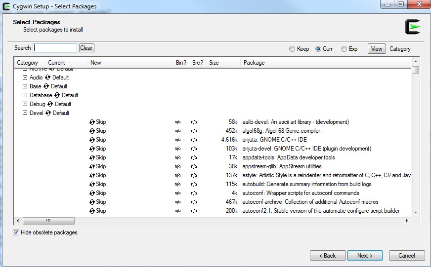
Scroll down the the devel menu and select the following packages:
binutuls
gcc core
g++
gfortran
gdb
make
You can also install all sorts of other things from cygwin like Ruby, Git and Python, but you don’t need to do that if you’ve already installed them. In fact, you might want to make sure git is not selected if you have installed the Git powershell from the github desktop application.
Once you have selected the things you need, select next. You might need to install a bunch of additional packages because your selected packages depend on them. If this is your first time installing cygwin go and get a drink or have lunch since installation will take some time.
C.3.3. C++ libraries
Some of our more specialized components require libraries. These are very difficult to install on Windows, and you will possibly self harm if you attempt to do so. Many of them are installed automatically using our vagrantfiles. Why don’t you make a Linux server with Vagrant instead?
C.4. GDAL windows installation
The <<LSDTopoTools vagrant setup installs GDAL for you on your Linux server. You also have GDAL python bindings if you follow our python instructions.
If you still really want a native version of GDAL (which is crazy, but it is your life), you can download GDAL for windows from this website: https://trac.osgeo.org/gdal/wiki/DownloadingGdalBinaries. If you are on Windows, however, you might want to just use the GDAL bindings
C.5. Ruby
Installing Ruby is only necessary if you want to play with our documentation, an perhaps add to it.
You can check to see if Ruby is installed on your system by typing
PS> ruby -vand you can check the Rubygems version with
PS> gem -vC.5.1. Install Ruby
-
Download and install Ruby: https://www.ruby-lang.org/en/documentation/installation/#rubyinstaller. We have used version 2.2.
-
Download and install Ruby Gems: https://rubygems.org/pages/download. To install this, you need to download it and then open a powershell window, navigate to the folder with gems in it, and run:
PS> \folder\with\rubygems\> ruby setup.rb -
Download the Ruby devtools: http://rubyinstaller.org/downloads/. You need to unzip this and run two things:
PS> \folder\with\DevKit\> ruby dk.rb init
PS> \folder\with\DevKit\> ruby dk.rb install
-
Now install bundler. In a powershell, you can, from anywhere, type
gem install bundler.
C.5.2. Fix rubygems on Windows
At the time of this writing, rubygems is "broken" on Windows: if you try to install a gem file you will get an error that says you cannot make an SSL connection. You will need to fix this problem by copying a trust certificate into you rubygems folder.
-
First download the file AddTrustExternalCARoot-2048.pem.
| It seems some browsers add formatting to this file when downloaded (Chrome does this, for example). I only managed to get this fix to work after downloading the file using Internet Explorer. |
-
Next, find the location of your gems installation:
PS> gem which rubygems
C:/Ruby21/lib/ruby/2.1.0/rubygems.rb-
Go to the folder and then go into the SLL_certs subfolder. In this case it is at:
C:/Ruby21/lib/ruby/2.1.0/rubygems/SSL_certs. Copy the.pemfile into this folder. Rubygems should now work.
C.5.3. Fix RubyDevKit on Windows
The devkit sometimes does not work the first time around. If you get error messages about the devkit, you should go to the devkit folder (you need to find it on your system) and run:
PS> ruby dk.rb initThis will generate a file called config.yml. Sometimes, the devkit installer will not find your Ruby installation, so you will need to add the path to your Ruby installation to this file.
For example, if your Ruby instalation is sitting in C:/Ruby21/, then you should modify the config.yml file to look like:
# This configuration file contains the absolute path locations of all
# installed Rubies to be enhanced to work with the DevKit. This config
# file is generated by the 'ruby dk.rb init' step and may be modified
# before running the 'ruby dk.rb install' step. To include any installed
# Rubies that were not automagically discovered, simply add a line below
# the triple hyphens with the absolute path to the Ruby root directory.
#
# Example:
#
# ---
# - C:/ruby19trunk
# - C:/ruby192dev
#
---
- C:/Ruby21/
C.5.4. Install some gems
From here we can install some useful ruby gems. Asciidoctor is really great for writing documentation. Bundler is useful for keeping Ruby packages up to date.
PS> gem install asciidoctor
PS> gem install bundler
C.5.5. If you use Ruby with Java (you will probably NOT need this)
This is for users who are trying to get a Ruby extension that uses Java installed. If you use an extension that need a java link, you will need the gem
PS> gem install rjb -v '1.4.9'But on my system this failed because you need to define the java runtime home. To do this, you need to figure out where your java installation is, and then define an environemnt variable $JAVA_HOME to point to this directory.
To do so, you should do this (in an administrator Powershell):
PS> [Environment]::SetEnvironmentVariable("JAVA_HOME", "C:\Progra~2\Java\jre_7_55", "Machine")Note that the powershell abbreviates Program files (x86) as Progra~2 and Program Files as Progra~1.
You can check to see if the appropriate path has been set with:
PS> Get-ChildItem Env:Unfortuately this only works in an administrator window.
C.6. Windows installation summary
If you actually managed to install things on Windows without permanent emotional scarring, I offer my sincerest congratulations. However, if you are just skipping ahead, why don’t you make your life easier and <<Installing LSDTopoTools using VirtualBox and Vagrant,use our (relatively) painless Vagrant setup>>? You should still install python, however.
C.7. Turning your windows machine into a Linux machine
The header of this section is a bit misleading, what you are really going to do is use software to create a virtual version of Linux within your Windows computer.
| Only do this if you want total control of your Linux enviroment. If you want us to do everything for you, read the instructions on Installing LSDTopoTools using VirtualBox and Vagrant and don’t continue reading this section! |
There are a number of options, popular ones include:
-
Parallels This software is proprietary.
-
VMWare There are several flavours of this. The free version is VMware Player.
-
VirtualBox This is open source.
Here I’ll walk you through setting up Linux using VMware. It just happened to be the one I tried first and it works, please do not take this as an endorsement. One disadvantage is it doesn’t seem to have an Apple version. If you use Apple you’ll need to try to go through a similar process using VirtualBox, which does have a version for Mac operating systems.
But, here is how you set up the VMware player. You will need a reasonable amount of storage (say at least 30GB: you will not be able to get this back!) and RAM (say at least 4 GB, but 8GB is better…note that this is only used when the virtual machine is on) A very old computer probably won’t work. If you’ve got a computer purchased in the last few years things will probably be fine. Note that the virtual machine permanently takes up some portion of your hard disk (you can release this protion back to your windows machine if you uninstall the virtual machine).
-
First, download VMware player. The download is currently here: https://my.vmware.com/web/vmware/free#desktop_end_user_computing/vmware_player/7_0.
-
Run the installation package. Brew a cup of tea while you wait for it to install. Maybe surf the internet a bit.
-
BEFORE you set up a virtual machine, you will need to download a linux operating system!
-
We are going to use Ubuntu, just because it is stable, popular and has good documentation. WARNING: I first attempted an installation with 64-bit Ubuntu, but it turns out my computer doesn’t allow guest 64 bit operating systems. To fix this I just downloaded the 32 bit version of Ubuntu, which worked. However, many of my students have sucessfully installed 65 bit Ubuntu.
-
Find the downloads link and download the latest version. It will be an
isodisk image. This will take a while. Put that time to good use.
-
-
Once that finishes downloading, you can set up your virtual box. First, open VMware Player.
These menus seem to change with new releases, so just try to pick the most sensible menu options if they don’t match the instructions. -
Now click on the "Create a New Virtual Machine" option.
-
-
It will ask you how you want to install the operating system. Tell it you want to use the Ubuntu disk image you just downloaded:
-
You will need to add some username information, and then you will have to pick a location for the Virtual Machine. I made a folder called
c:\Ubuntufor it: -
Now allocate disk space to the virtual machine. This disk space cannot be used by your windows operating system!!. I decided to use a single file to store the disk since it should be faster.
-
The next page will say it is ready to create the virtual machine, but it has a default Memory (in my case 1 GB) allocated. I wanted more memory so I clicked on the customize hardware button: This allowed me to increase the memory to 2GB.
Memory will be used when the virtual machine is on, but when not in use the memory will revert to your original operating system. You can change the amount of memory allocated to your virtual machine by changing the virtual machine settings from the VMware start page. The size of the DEM you can analyse will be limited by your memory. Give the virtual machine as much memory as you can spare if you are running analysis on big DEMs. -
You might be asked to install some VMware Linux tools. You should do this, as some things won’t work if it isn’t installed.
-
Installing the operating system within the virtual machine will take ages. You might schedule this task for your lunch hour, which is what I did. My chicken shawarma wrap was delicious, thank you for asking.
-
When Ubuntu has installed, it will look for software updates. You should install these. This will also take ages. Maybe you have a book to read?
-
Finally, you should be aware that the default keyboard layout is US. Getting UBUNTU to recognize a different keyboard is a bit of a pain.
-
First go to system settings.
-
Then click on language support.
-
It will need to install some stuff.
-
Go to text entry.
-
In the lower left corner click on the
+button. -
Add your country’s input source.
-
C.8. Summary
By now you should be able to pull up a powershell and call the essential programs we will be working with in this course.
Appendix D: Setting up on Linux
| These instructions involve building your own operating system with a virtual machine. You can do this if you want more control, but most users should follow the simpler process of creating an lSDTopoTools server using Vagrant. Instructions can be found here: Installing LSDTopoTools using VirtualBox and Vagrant. |
Setting up your system on Linux is considerably easier than setting up on Windows.
Before doing anything, open a terminal window. The $ symbol below indicates commands typed into the terminal window.
In Ubuntu, the terminal window is opened with ctrl+alt+T. You can also find it in the applications menu under accessories.
| These commands are for Ubuntu and Debian flavors of Linux. Other flavors of Linux use different package managers, such as yum. If you don’t use Debian of Ubuntu, you will need to look up the installation guidelines for the programs below. |
| It is MUCH easier to run LSDTopoTools software in Vagrant server (basically because we install everything for you), but you should install programs for looking at your data (i.e., python, a GIS) on your host operating system (in this case your desktop version of Linux, versus the Linux server run by vagrant). In the case of Linux if you do install natively it will run faster than if you use a Vagrant server. |
D.1. A text editor
We recommend Brackets:
$ sudo apt-get install bracketsNote that this will only work with a windowing system (i.e., not on a server-only version of Linux).
D.2. Git
To check if git is working, type
$ git --versionIf it isn’t installed, install it with
$ sudo apt-get install gitD.3. C++ tools
You can check if these are working by typing (this assumes you are using the GNU compilers)
$ g++You can install these with
$ sudo apt-get install g++These seem to install gdb and make, which is convenient.
D.3.1. C++ libraries
For more specialized versions of the code, you will need some libraries. Installing these can sometimes be tedious, sou you might want to wait until you actually need them before you install.
Spectral analysis: the easy way
Any analyses that use the RasterSpectral objects, which includes the LSDRasterModel, require the fast fourier transform libraries. In the source code, you will find #include statements for these libraries, and corresponding library flags in the makefile: -lfftw3. In the LSDTopoTools packages that use FFTW, we include the correct header along with the source code so you shouldn’t have to worry about that.
Installation using sudo should be fairly easy. On Ubuntu just run:
$ sudo apt-get install fftw3Debian should have a similar installation package.
Spectral analysis: the hard way
If you want to compile FFTW yourself, you can go here: http://www.fftw.org/download.html
Installation should be fairly easy, but occasionally doesn’t work. It also leave a load of files on your system that you don’t need. Go to the FFTW download folder and run:
$ ./configure
$ make
$ make installThe landscape evolution model
Boost. Boost contains a large number of header only libraries. You will need to know where you have unzipped them! But the good news is that you don’t need to install anything.
More information is here: http://www.boost.org/doc/libs/1_59_0/more/getting_started/unix-variants.html
The Matrix Template Library version 4 is also requires: this does some heavy duty computation on sparse matrices that is required for the landscape evolution model.
You can get download and installation instructions here: http://www.simunova.com/node/189
D.4. The Swath and Point Cloud tools
As mentioned in previous sections, these tools require the use of the following libraries and tools, which themselves come with further dependencies.
-
The
cmakeutility. This is likemakebut is required for our tools that examine point clouds, since it is required by something called the point cloud library. -
pcl: The Point Cloud Library.
-
libLAS: a library for working with LAS format data.
D.4.1. PCL
Before you can install PCL however, it itself is dependent on some other things…
-
blas (blas-devel)
-
eigen3 (eigen-devel)
-
flann
-
libLAS
PCL, blas-devel, flann, eigen3 etc. can be installed in linux using the yum or apt-get commands in many distributions:
yum install blas-devel flann-devel eigen3-devel pcl-develYou will need to check the exact names of these packages in your package repository manager first.
If you can’t install using the above method, you will have to do a manual install following the instruction on the relevant websites. The PCL website is a good place to start for guidance.
After installing these, you may run into the further problem that the location of the libraries on your system are not where the compiler thinks they are, because the installation folders are named by the version number, e.g. /pcl-1.7.2 rather than just /pcl. You can get around this by creating symbolic links to these folders. From the include directory on your system, (mine was /usr/include/), type:
ln -s /usr/include/pcl-x.x.x /usr/include/pcl- and the same goes for the
eigenlibrary
ln -s /usr/include/eigen3 /usr/include/EigenRight, we are nearly ready to go!
Except for the last library dependency…
D.4.2. libLAS
If you thought installing pcl was a faff, libLAS takes things to a new level. It isn’t included in most linux distribution package repositories, so you have to install it manually. Do not confuse it with the similarly named Blas or libblas, which ARE in the linux pacakge repositories but have nothing to do with the libLAS that we want (BLAS is a basic linear algebra library).
First of all, it is dependent on the libgeotiff-devel library, so go ahead and install that using yum or apt-get:
yum install libgeotiff-develIt can be a good idea to update the library paths in linux at this point:
sudo ldconfigGreat. Now libLAS is also dependent on another package called laszip. The developers thought it would be too easy to simply include this as one package/download, so you first have to install this as well before we can even get started on the actual libLAS package.
Get it here: laszip download
Once you’ve unzipped it, in the top level directory run:
./configure
make
sudo make installThey should be installed in the /usr/local/include/ directory. Which is bad, because they need to be in their own directory. So you have to root into the /usr/local/include/, create a laszip directory, and copy the laszip header files into this directory.
Magic. Now, we can install libLAS. It uses cmake to install itself. So in the libLAS directory, mkdir a build folder, cd into that, and run:
ccmake -G "Unix Makefiles" ../A terminal dialogue opens. Make sure it has found the GEOTIFF directory. If not, you will need to find where the geotiff (see above) stuff was installed to, and enter the full path in the GEOTIFF box.
Now look at the options below (we are still running ccmake here). Turn all the optional settings to OFF, it just makes things easier and less likely to go wrong during compilation. Hit configure. Save and exit.
Now run:
make
sudo make installHopefully, cmake should do its thing and install libLAS for you. If not, open a large bottle of whisky and repeat the above steps to check you haven’t missed anything. I find a peaty single malt works best here.
D.5. Python
To check if it is working, just type
$ pythonIf it is working, it will tell you the version and you will get a command prompt that looks like this:
>>>You should have version 2.7 or above. Our python plotting scripts are based on python 2.7 so you should probably have a version of that installed.
D.5.1. Installing python
If you don’t have python, you should install both python and pip, which manages python packages. To do that type:
$ sudo apt-get install python2.7
$ sudo apt-get install python-pipD.5.2. Installing python packages
To check if python packages are there, just try to import them. First start a python session:
$ pythonThen, try to import a package. For example:
>>> import matplotlibIf the package does not exist, you will get an error message like this:
Traceback (most recent call last):
File "<stdin>", line 1, in <module>
ImportError: No module named matplotlibYou can install all the packages at once with:
$ sudo apt-get install python-numpy python-scipy python-matplotlib ipython ipython-notebook python-pandas python-sympy python-noseYou can upgrade packages with the pip command:
$ pip install PackageNameHere --upgradeD.5.3. Installing python with miniconda
Native Linux users will probably want to do things using pip (see below) but you can also use miniconda. First install miniconda using instructions here. We will use Python 2.7, so use the Python 2.7 installer. Then use the conda command to install stuff:
$ conda install scipy
$ conda install matplotlib
$ conda install pandas
$ conda install gdal
$ conda install spyderTo run spider you just type spyder at the command line.
Warning: Spyder needs an older version of a package called PyQt. If spyder doesn’t start correctly, run conda install pyqt=4.10 -f
Note that spyder will only work if you have a windowing system (i.e., you can’t use it via a ssh connection).
D.6. QGIS
You might want to look at your data in a GIS, and [http://www.qgis.org/en/site/]QGIS is a nice open-source option. Linux installers are on the QGIS downloads page. You will need a windowing system for this (i.e., you can’t do it on a server-only version of Linux).
D.7. Inkscape
Many of our python plotting scripts can output figures in svg format, which you can then edit in Inkscape, an open source editor that is similar to Illustrator. Inkscape also is happy with .ai, .pdf and .eps files.
You can install with
$ sudo add-apt-repository ppa:inkscape.dev/stable
$ sudo apt-get update
$ sudo apt-get install inkscapeYou will need a windowing system for this.
D.8. Ruby
As mentioned in the main section of the book, the ruby programming language is used to build the documentation of our software. You can skip this part if you are viewing the documentation from the pdf or webpages and aren’t planning on contributing to the documentation. (Though you if you are contributing new features to the software you are encouraged to!)
You can see if Ruby is on your system by typing:
$ ruby -vIf it isn’t there, install with (this should seem routine by now):
$ sudo apt-get install ruby-fullIf you already have ruby installed, you might need to check you have the development packages too, along with rubygems, which is a package installer for ruby libraries and add-ons (similar to pip for Python):
$ sudo apt-get install ruby-dev
$ sudo apt-get install rubygemsNote that in newer versions of Ruby, rubygems seems to install with ruby-full.
D.8.1. Installing the asciidoctor documentation software
After you have installed ruby, ruby-devel, and rubygems you can now proceed to getting the actual ruby packages that make the documentation:
$ sudo gem install asciidoctor
$ sudo gem install bundlerIf bundler fails to install, you may be missing the ttfunk package.:
$ sudo gem install ttfunkThankfully, the gem installer is quite helpful at telling you which packages are missing and how to quickly install them. That’s it now, you can proceed to cloning the documentation from github.
D.9. Cloning or forking the documentation
The documentation is under version control on github, just like the actual software source code. If you’re a developer, you can clone it direct from the original repository, otherwise you will need to fork it first into your own repo, and then clone from there to your local machine. You do this by visiting http://github.com/LSDtopotools/LSDTT_book and clicking 'fork' (assuming you have a github account of course). Then, on your local machine, you can do:
$ git clone https://github.com/LSDTopoTools/LSDTT_book.gitand the documentation will be cloned into a directory called LSDTT_book from where you ran the command.
cd into the LSDTT_book directory, and run bundler install:
$ bundler installThen, to build the documentation in full from the source files, run:
$ bundler exec rake book:buildor to just build html:
$ bundler exec rake book:build_htmlIn a few seconds bundler will have completed and you will have a smart looking copy of the documentation in both pdf and html form. Any time you make changes to the documentation source files, run the bundler exec command again to update your local copy. Remember to commit and push your changes regularly to the remote repository on your githb account.
D.10. Summary
Well, you have probably spent some time installing all of these software packages so relax for a bit and enjoy the beverage of your choice!
Appendix E: Setting up on MacOS
It is possible to run LSDTopoTools natively on MacOS, because they run on Linux and MacOS is built on top of Linux. However, we are not even going to tell you how to do that since it is 1000x easier just to set up a Linux server in your MacOS machine using Vagrant. Instructions can be found here: Installing LSDTopoTools using VirtualBox and Vagrant.
E.1. Looking at the data
If you have used our instructions on setting up using Vagrant, then your MacOS machine will be able to see files (rasters, point data, paramfiles) generated by you Linux server. To look at these you should have:
-
A GIS. QGIS is a good, ope-source GIS. You can download it from here
-
Python. We strongly recommend using miniconda to install python. Our plotting scripts use Python 2.7 so you should download that one. Once miniconda is downloaded, go into a terminal window and run the following:
$ conda install scipy $ conda install pandas $ conda install matplotlib $ conda install gdal $ conda install spyder $ conda install pyqt=4.10 -fThe last command is because spyder and matplotlib use conflicting versions of something called PyQt (as of September 2016).
-
A text editor. We recommend Brackets but there are many other choices. Atom also works on MacOS.
| Even though QGIS and python both have Linux installers, don’t install them on your Linux server for use with LSDTopoTools. This is because we use these programs to look at data, and our vagrant server cannot produce windows. You should do this n your native operating system. |
Appendix F: Code Structure
You can happily use LSDTopoTools oblivious to the inner-workings of the code and how it all connects together to produce a suite of topographic analyses at your disposal. Ignorance is, as they say, bliss. No knowledge of Classes, Drivers, Objects, and so on, is needed to run the basic analyses supplied in the distribution of this software. However, you might wish to write your own driver functions, and may even be considering contributing to the core parts of the code. This way you can make your topographic techniques and algorithmic awesomeness available to like-minded geoscientists. Earlier, we mentioned breifly how the code is structured in the main body of this documentation. For those intrepid interrogators of empirical inquisition who have made it four levels down into the Appendix section, first of all, we salute you, and we reward you with a deeper look into how the code is structured, should you wish to contribute your own additions to the repository.
F.1. Source Files: Drivers, Headers, and Implementaions.
There are two main parts of the LSDTopoTools source code: the driver functions and the core component source files. The core files contain the implementations of topographic analyses, and many other functions for creating rasters, sorting data, performin file operations, writing output, and so on. All the core source files are name like LSDSomeFile. pp. They also come in pairs: a LSDSomeClass.cpp source file comes with a LSDSomeClass.hpp header file. The header file describes the interface to a parituclar source file. In other words, LSDSomeClass.hpp tells us what all the methods and data structures of a particular source file (LSD.cpp) are. For functions (or class methods to be precise…) the header file tells us what type of parameters the functions take as arguments, and what data types (if any) these functions return. They also describe how data structures are stored. For example, we could look in LSDRaster.hpp to see how the data members of a Raster are defined. We would see that an LSDRaster object has some meta-data telling us about the extent and coordinates of the the raster data, and an array that stores each pixel value in the raster. It would also tell us which functions (methods) would return information about the LSDRaster object. If we wanted to know the number of rows in a raster object we would see in the header file there is a getNRows() function, and so on. The .cpp files tell us how these functions are implemented, e.g. what exactly each function does when parameters are passed to it, and how it maniplulates the data stored with the object.
In general, although it is not required, we have kept one Class to one pair of header and implementation files. (Although there are a couple of exceptions to this). So in the LSDRaster.hpp and LSDRaster.cpp core files, you will find the declaration and implementation of the LSDRaster class, respectively. In short, hpp tells us what is there and how to use it, cpp tells us how it works. For a full description of all the LSDTopoTools objects and classes you can visit the automatically generated doxygen documentation.
The driver files are separated off into their own folder(s) and as their name suggests, they are responsible for driving a particular analysis by calling on different objects and functions defined in the core source files. The core LSDFooBar-type files we talked about previously don’t actually do much on their own — they are just a bunch of class data structures and methods. This is where the driver files come in: driver files are written to perform a certain kind of topographic analysis or model simulation using some form of input data created by you, the user. Driver files call upon different parts of the object files to perform topographic analyses. An example driver file may call upon LSDRaster to create a Raster object to store data from an input DEM, then it might pass this LSDRaster object to LSDFlowInfo to calculate the flow routing paths in the raster, and so on, until we have completed a useful analysis and written some output data to analyse.
Since there is such a variety of functions defined in the source code, there are potentially hundreds if not thousands of possible analyses that could be performed with the code. The driver files provided with the TopoTools distribution are designed to accomplish some of the more common topographic analysis tasks, e.g. extracting basins from a raster, calculating the location of channel heads in a landscape, running a chi-analysis on river channels, or extracting swath profiles, and so on. However, you are free to write your own driver files of course! What’s more, they provide an exact record of the analysis you have just done, and so are inherrently reproducible if you want to share your findings with others.
Another way to think of drivers, if you are familiar with C or C++ programming, is that they contain the int main() { } bit of a typical program. I.e. the main workflow of a program.
|
F.2. A closer look at the source files
F.2.1. LSDRaster
LSDRaster is the class that contains methods for mainipulating arrays of raster data loaded from a DEM file. There are also data members that store metadata about the raster, such as the typical header data you would find in a DEM file. It can perform typical analyses such as creating a hillshade raster, calculating curvature of ridgetops, calculating the location of channel heads in a landscape, filling sinks and pits in a DEM and so on — mainly analyses that are performed on the entire raster dataset. It also does the basic reading and writing to DEM files.
F.2.2. LSDIndexRaster
A simple and fairly short class that stores rasters data as integers, used for indexing of raster data, calculating bounding boxes for rasters with lots of NoData values around the edge (or surounding basins). Very similar to LSDRaster class except is only used for when an index or mask of a given raster is needed.
F.2.3. LSDFlowInfo
This class performs operations such as calculating flow direction, calculating upstream contributing pixels in a raster, calculating sources based on threshold pixel methods, and other flow related information (based on topographic analysis — not based on any particular hydrological fluid flow calculations). Note how this object has include statements for LSDRaster and LSDIndexRaster — it returns these type of objects from many of its methods. It uses the FastScape algorithm of Braun and Willet (2014).
F.2.4. LSDIndexChannel
This object contains the node indexes as well as the row and col indices for individual channel segments.
F.2.5. LSDChannel
LSDChannel is our first class that inherits the public methods and data members of another, namely LSDIndexChannel. This means we have direct access to the public members of that class. Note, in the source code:
class LSDChannel: public LSDIndexChannel
{
public:
// Some method declarationsIndicates this class inherits from LSDIndexChannel. LSDChannel stores information about the actual channel characteristics, e.g. elevation etc.
F.2.6. LSDJunctionNetwork
JunctionNetwork contains the main parts of the implemented FastScape algorithm for creating channel junction networks that can be searched for network connectivity. The main inputs are a FlowInfo object and list of source nodes. It also contains functions for returning IndexChannel objects after calculating the layout of channel networks.
F.2.7. LSDIndexChannelTree
This object spawns vectors of LSDIndexChannels. They can be indexed by the LSDChannel network, but can also be independent of the channel network, storing longest channels from sources, for example. The class is designed to be flexible, it can be used either with the LSDFlowInfo or LSDJunctionNetwork classes.
F.2.8. LSDChiNetwork
This is used to perform chi-related analyses on channels.
F.2.9. LSDMostLikelyPartitionsFinder
This object is principally used to identify segments of differing channel steepness in chi-zeta space. It contains the implementation of the segment fitting algorithm, including the statistical model that determines the most likely partitionining combination of channels.
F.2.10. LSDStatsTools
The StatsTools files contain a number of classes and standalone functions that perform statistical analyses. A number of other utility functions are implemented here, such as file name parsing and formatting.
Appendix G: Analysis Driver Options
LSDTopoTools is composed of a number of objects (e.g., LSDRaster, LSDChannel, LSDFlowInfo, etc.) which are then called from programs we call driver functions. For more information, see the appendix Code Structure.
Most of these functions drive specific kinds of analysis, but we do have a general program capable of a number of different analyses. This program is called the AnalysisDriver and is available here: https://github.com/LSDtopotools/LSDTopoTools_AnalysisDriver.
The analysis driver runs from parameter files. In this appendix we document the options for running the AnalysisDriver from a parameter file.
The format of AnalysisDriver parameter files is a keyword followed by a value.
The value can be a string, an integer, a boolean or a floating point number depending on the keyword.
The order of the keywords does not matter.
Comments can be inserted into the parameter file using the hash symbol (#).
G.1. AnalysisDriver file input and output options
| Keyword | Input type | Description |
|---|---|---|
dem read extension |
string |
The type of data format used in reading rasters. Options are |
dem write extension |
string |
The type of data format used in reading rasters. Options are |
write path |
string |
The path to which data is written. |
read path |
string |
The path from which data is read. |
write fname |
string |
The prefix of rasters to be written without extension.
For example if this is |
read fname |
string |
The filename of the raster to be read without extension. For example if the raster is |
G.2. AnalysisDriver files to write
These require booleans,
but in in the AnalysisDriver parameter file booleans must be true--anything else is considered false.
true is case sensitive, so DO NOT write True: it will be interpreted as false!!
|
| Keyword | Input type | Description |
|---|---|---|
write fill |
boolean |
Write a filled raster. |
write write trimmed and nodata filled |
boolean |
This is for data with nodata around the edges and holes of nodata in the middle. The holes are filled and the nodata around the edges is trimmed. |
write hillshade |
boolean |
Write a hillshade raster. |
write mask threshold |
boolean |
Write a masked raster. This will contain the original data but data above or below a threshold (you decide which one using other parameters) is changed to nodata. |
write curvature mask threshold |
boolean |
Write a mask raster based on curvature. This doesn’t retain the curvature values, but rather yeilds nodata if you are obve or below a threshold (you set that with a parameter) and otherwise 1. |
write slope |
boolean |
Write a slope raster. |
write curvature |
boolean |
Write a curvature raster. |
write planform curvature |
boolean |
Write a planform curvature raster. |
write tangential curvature |
boolean |
Write a tangential curvature raster. |
write profile curvature |
boolean |
Write a profile curvature raster. |
write aspect |
boolean |
Write an aspect raster. |
write topographic classification |
boolean |
Write a raster where convex, concave and planar regions are classified by an integer. |
write drainage area |
boolean |
Write a drainage area raster. |
write channel net |
boolean |
Write a channel network. This will print a raster of stream orders and a raster of junctions. |
write nodeindex |
boolean |
Writes a nodeindex raster. Used by developers for debugging. |
write write single thread channel |
boolean |
This extracts a single tread channel from a starting and ending node, and prints to csv. |
write chi map |
boolean |
This calculates the chi coordinate (a coordinate that integrates drainage area along channel length) from all base level nodes. |
write factor of safety at saturation |
boolean |
Calculates the factor of safety using an infinite slope analysis (similar to Sinmap or Shalstab). |
G.3. AnalysisDriver parameter values
G.3.1. Parameters for the fill function
| Keyword | Input type | Default | Description |
|---|---|---|---|
min_slope_for_fill |
float |
0.0001 |
The minimum slope between nodes in a DEM: this is for filling flats |
fill_method |
string |
new_fill |
The method to be used for the fill function. Options are |
G.3.2. Parameters for hillshading
| Keyword | Input type | Default | Description |
|---|---|---|---|
hs_altitude |
float |
45 |
The altitude of the sun in degrees |
hs_azimuth |
float |
315 |
The azimuth of the "sun" in degrees |
hs_z_factor |
float |
1 |
The vertical exaggeration factor as a ratio |
G.3.3. Parameters for flow info calculations
| Keyword | Input type | Default | Description |
|---|---|---|---|
boundary conditions |
A four element list of strings |
n n n n |
This gives the boundary conditions at the north, east, south and west boundaries, respectively.
The options are |
G.3.4. Parameters for masking
| Keyword | Input type | Default | Description |
|---|---|---|---|
curvature_mask_nodataisbelowthreshold |
int |
1 |
This works like a boolean. Anything other than 1 is treated as false. If true, anything below the threshold is masked (i.e., turned to nodata). If false anything above threshold is turned to nodata. |
curvature_mask_threshold |
float |
0 |
A threshold value of curvature from which to derive the mask |
mask_nodataisbelowthreshold |
int |
1 |
This works like a boolean. Anything other than 1 is treated as false. If true, anything below the threshold is masked (i.e., turned to nodata). If false anything above threshold is turned to nodata. |
mask_threshold |
float |
0 |
A threshold value from which to derive the mask of nodata values. |
G.3.5. Parameters for chi calculations
| Keyword | Input type | Default | Description |
|---|---|---|---|
A_0 |
float |
1000 |
A normalizing area for chi calculations in m2. This will affect absolute values of chi but not relative values of chi. |
m_over_n |
float |
0.4 |
The m/n ratio. |
threshold_area_for_chi |
float |
0 |
Threshold area for chi calculations in m2. Pixels with area lower than this threshold will be assigned nodata. |
G.3.6. Parameters for polyfit and slope calculations
| Keyword | Input type | Default | Description |
|---|---|---|---|
polyfit_window_radius |
float |
2*sqrt(2)*data_resolution |
The radius of nodes over which to fit the polynomial window in m. |
slope_method |
string |
d8 |
The method for calculating slope. Options are |
G.3.7. Parameters for drainage area extraction
| Keyword | Input type | Default | Description |
|---|---|---|---|
drainage_area_method |
string |
dinf |
The method for calculating drainage area. The options are: |
G.3.8. Parameters for single thread channel extraction
| Keyword | Input type | Default | Description |
|---|---|---|---|
single_thread_channel_method |
string |
start_and_end_node |
The method for calculating drainage area. So far there is only one option: |
starting_channel_node |
int |
if none give you will get a user prompt |
The nodeindex of the starting node. |
ending_channel_node |
int |
if none give you will get a user prompt |
The nodeindex of the ending node. |
G.3.9. Parameters for area threshold channel extraction
| Keyword | Input type | Default | Description |
|---|---|---|---|
pixel_threshold_for_channel_net |
int (but in program seems to be float…need to check) |
The number of pixels that are needed to initiate a channel. |
G.3.10. Parameters for hydrology and slope stability
| Keyword | Input type | Default | Description |
|---|---|---|---|
root_cohesion |
float |
The root cohesion in N m-2. |
|
soil_density |
float |
The soil density in kg m-3 |
|
hydraulic_conductivity |
float |
The hydraulic conductivity in m day-1. |
|
soil_thickness |
float |
Soil thickness m (assumed to be the same everywhere). |
|
tan_phi |
float |
0.8 |
The friction angle (dimensionless). |
Appendix H: DEM preprocessing Options
The DEM preprocessing program is distributed with the AnalysisDriver and can be found here: https://github.com/LSDtopotools/LSDTopoTools_AnalysisDriver.
Like the analysis driver, the DEM proprocessing program runs from parameter files. In this appendix we document the options for running the DEM preprocessing program from a parameter file.
H.1. AnalysisDriver file input and output options
| Keyword | Input type | Description |
|---|---|---|
dem read extension |
string |
The type of data format used in reading rasters. Options are |
dem write extension |
string |
The type of data format used in reading rasters. Options are |
write path |
string |
The path to which data is written. |
read path |
string |
The path from which data is read. |
write fname |
string |
The prefix of rasters to be written without extension.
For example if this is |
read fname |
string |
The filename of the raster to be read without extension. For example if the raster is |
H.2. DEM preprocessing routines to run
These require booleans,
but in the parameter file booleans must be true--anything else is considered false.
true is case sensitive, so DO NOT write True: it will be interpreted as false!!
|
| Keyword | Input type | default | Description |
|---|---|---|---|
fill_nodata |
boolean |
false |
Fills holes of nodata in a DEM |
remove_low_relief |
boolean |
false |
Finds low relief areas (defined by parameters below) and sets to nodata. |
write_relief_raster |
boolean |
false |
Writes a relief raster. |
H.3. Parameters for removing high and low values (including weird nodata)
| Keyword | Input type | default | Description |
|---|---|---|---|
minimum_elevation |
float |
0 |
The minimum elevation of the DEM. Anything below this is set to nodata. |
maximum_elevation |
float |
30000 |
The maximum elevation of the DEM. Anything above this is set to nodata. It is set to 30000 to account for yanks, who bizarrely insist on using idiotic Imperial units, even though everyone else in the world realised decades ago that they are crap. |
H.4. Parameters for masking parts of the DEM
| Keyword | Input type | default | Description |
|---|---|---|---|
filling_window_radius |
float |
50 |
Radius of the window that is used to search for nodata islands. If there is a non nodata point withing this radius of a nodata point it is filled. |
relief_radius |
float |
100 |
Radius of the window over which relief is calculated. |
relief_threshold |
float |
20 |
Any relief less than this will be turned to nodata. |
Appendix I: Tools for viewing data
The many analyses provided by LSDTopoTools produce geographic data (that is data that is attached to some location in space). In this section we provide some basic instruction on how to view this data, using either Geographic Information Sysems (GISs) or using our own visualisation scripts, which are written in python.
I.1. ArcMap
ArcMap is commercial software written by ESRI. Many companies, goverment agencies and universities have liscences to this sofotware.
I.2. QGIS
QGIS is an open source GIS that has functionality similar to ArcMap.
I.3. LSDTopoTools python mapping functions
We have written a series of lightweight mapping tools in python for visualising data. These tool are for times when you cannot be bothered waiting for a GIS to load, or when you want a perfectly reproducable, code-driven visualisation.
To make these work, you will need matplotlib and the gdal python packages installed on your system.
I.4. Summary
You should now be able to perform basic operations such as loading and exploring data in QGIS, ArcMap or our own python tools.
Appendix J: Automation and Supercomputing for LSDTopoTools
Perhaps you have a lot of basins that you want to perform some analysis on, or you want to re-run a previous analysis with slightly different paramters, different m/n values, and so on. This section will explain some of the scripting tools, supercomputer applications, and other utilities to help speed up this process.
J.1. Embarassingly Parallel Topographic Analysis
The LSD software is written to run completely in serial. (i.e. there is no built in parallelisation). However, if you are running the same analyses on a large number of basins, the problem becomes easy to set up in a parallel-like fashion, if you have access to some form of multiple cpu computing facility. (This is termed embarassingly/trivially parallel, since it isn’t really written in parallel code).
This doesn’t necessarily require a supercomputing cluster; most laptops are at least dual core (as of 2014), and some will have as many as 8 seperate cpu threads to run tasks on. That means you could be running analysis on 8 basins at a time, rather than waiting for each one to finish separately, in serial.
J.1.1. The Simple Case - A single cpu, multi-core laptop
- You can find out how many cpus/cores/threads you have to play with by typing
nprocat the terminal in linux/cygwin. On a Intel i5 laptop, for example, it would probably return 2 or 4 'cpus' as the result. Without going into the details, a 'cpu' in this case is the smallest processing 'unit' (or a 'thread'). Also, by means of some clever electronics, some Intel cpus have twice as many threads as they do physical cores. Hooray!
Now suppose you have 16 basins that you want to do the chi analysis on. Should you run them all one-by-one on a single thread/cpu and let the other 3 threads sit there idle-ing? No! Use a utility such as xjobs or GNU Parallel. This example uses GNU parallel:
Prepare your numbered driver files as required. This example uses 50 driver files named: test1.driver, test2.driver, etc. (See below for how to do this with a Python Script). The job-queuer used is GNU parallel, which is installed by default on many linux distributions:
seq 50 | parallel --gnu -j 4 ../driver_functions ./ 'test{}.driver' &or,
parallel --gnu -j 4 ../driver_functions/chi_get_profiles.exe ./ test{}.driver {1..50} &This will queue up you 50 separate jobs to run on 4 threads at a time (the -j 4 argument)
J.2. Topographic Analysis on a Supercomputer
If you have access to a suitable cluster computer or other supercomputer (HPC - high performance computing) service (ARCHER, HECToR, Eddie, or your local department’s cluster) it will probably have some type of job submission service. SGE and PBS are two of the most commonly used ones. You use the job scheduler to submit your by providing a simple script that requests cpu and memory resources from the supercomputer. By running the script, the job(s) are then placed in a queue to be distributed across the nodes and cpus.
It is also possible to run jobs in 'interactive' mode, which skips the script writing part and just starts the jobs from the commmand line once you are logged in. This is ok for testing, but not advised when running large, numerous, or memory-intensive jobs as it tends to hog the resources. Consult your HPC service’s documentation for best practice.
J.2.1. Launching jobs with the batch system
PBS Example
PBS (Portable batch system) is the name of the job submission scheduler used on the UK’s ARCHER supercomuting service, housed in Edinburgh.
Here is an example of a batch of channel file extractions. 50 channel files were extracted in a few minutes, compared to several hours on a desktop/laptop computer.
#. First, set up your driver files using the python script described above. Upload them to the filesystem on the HPC service.
#. Upload (using scp) and compile the LSD Topo Tools software directly on the HPC system. I.e. do not upload it ready-compiled from your own computer, it will probably not work - unless you have compiled it with static libraries. (This is not the default option)
#. Upload any raster files required for whichever part of the LSD ToolBox you are using. You would normally do this using the linux scp command. Type man scp at the terminal for help on using this.
#. Now write the job submission script. The example below is for the PBS job submisison utility, but SGE has a very similar layout. See specific documentation for the one you are using.:
#!/bin/bash --login
#
#PBS -N chan_extrac
#PBS -A n02-ncas
#PBS -l walltime=2:0:0
#PBS -l select=serial=true:ncpus=1
#PBS -J 1-50
#PBS -r y
# Switch to current working directory
cd $HOME/wasatch_chi/channel_extraction_legacy/new_dense_chans/
# Run the serial program
../driver_functions/chi2_write_channel_file.exe ./ wasatch_$PBS_ARRAY_INDEX.driverThis is an array job: the array switch is specified by #PBS -J {RANGE OF VALUES}. The range will increment the variable $PBS_ARRAY_INDEX by 1 each time. In this example, the driver files used will be wasatch_1.driver, wasatch_2.driver, …, and so on.
Since the job (jobs) are all written in serial code, there is no need to run this on parallel nodes, should they be available to you. This is specified here with #PBS -l select=serial=true:ncpus=1, since we only need one cpu for each individual job in the array. (Altough they will all run concurrently on multiple cpus).
There is no need to specifiy an output pipe. Screen output and any errors/aborts will be written to log files automatically.
Submit the array job using:
qsub my_array_script.pbsThe status of the jobs can be checked using qstat. (See the separate documentation for this, or just type 'man qstat')
SGE Script Example
SGE (Sun grid engine) is used on the Eddie cluster (Edinburgh) and Redqueen (Manchester). It works much the same way as PBS does. Here is an example script used to perform the chi analysis on the 50 channels we extracted in the previous example.
#!/bin/bash
#$ -S /bin/bash # Inform SGE we are using the bash shell
#$ -cwd # Job will run in the current directory (where you ran qsub)
#$ -V # Inherit current environment (e.g., any loaded modulefiles)
#$ -q atmos-b.q # tell qsub to use the atmosci-b queue
#$ -t 1-50 # TASK GRID ARRAY with 50 jobs
../bin/chi_analysis.exe ../data_dir/ inputfile.${SGE_TASK_ID}.parametersThe ${SGE_TASK_ARRAY} part will increment by 1 across the sequence specified, so make sure your inputfiles conform to this format. e.g.
inputfile.1.parameters
inputfile.2.parameters
inputfile.3.parameters
{etc...}The job is submitted using qsub my_batch_job.sh. In similar fashion to the previous example, we are submitting a task grid array job, which is useful for carrying out sensitivity analysis (such as with the chi-analysis tools). The chi software is not written with any parallelisation, but we can simulate the effect here using multiple cpu threads on the cluster computer with the task-grid-array job.
In this example, we specified a particular queue to use: -q atmos-b.q. This is not necessary on some systems, so check the documentation first.
J.2.2. Checking your jobs
qstat on its own should display a list of all your running jobs by default. To delete a job, use:
qdel -j {JOB_ID_NUMBER}The job ID number is found from qstat. To delete all your jobs, use:
qdel -u {USERNAME}To delete specific tasks from an array of jobs (like in the above examples, use:
qdel -j {JOB_ID_NUMBER} -t {TASK_NUMBER(S)}So if you want to delete the tasks 23 through 64 from job ID 1300. Use:
qdel -j 1300 -t 23-64J.3. Module issues
On certain HPC services, different modules or libraries need to be loaded or switched to create the right environment to run your software. Normally this is not an issue and nothing needs to be changed. By convention, the LSD Topo Tools software is compiled using the gcc compilers. (A set of free compilers released under the GNU licence). Some supercomputer clusters will come with a range of compilers such as Intel, Cray, etc… One of them will be loaded by default. If gcc is not the default, you may wish to swap it before compiling.:
module listWill list all the currently loaded modules:
module availWill list the available modules. You can narrow down your search by doing:
module avail gccfor example, to find the gcc-releated modules. To load, type module load gcc. If you are swapping modules, for example the Intel compiler for the gcc one, then do:
module swap intel gccSometimes, you may find that there is a ready-to-use compiler suite/environment set up on your HPC. Such as:
PrgEnv-intel
PrgEnv-gnu
PrgEnv-crayLoading or swapping one of these is the equivalent of the above, but loads a whole suite of other modules and libraries that match the compiler suite. It is probably best to use these if they are available.
| The compiler suite you use has nothing to do with the type of CPU or supercomputer manufacturer. So you don’t have to use the Cray compilers with a Cray supercomputer, for example. You may also find that the LSD Topo Tools compile perfectly fine using the Intel/Cray/whatever compilers, though we have only tested the code using the GNU/gcc ones. |
Other modules that may of interest to LSDers include python (though not all HPCs will have an implementation installed.) netCDF (a data format for large data arrays).
J.4. Compilation and library issues
| This may not be an issue on certain cluster systems. I include it here in case anyone is having similar issues. |
Users of certain libraries (some of the fast fourier libraries, very new compiler features, etc.) may find that the libraries they have on their personal systems are not availble on the cluster computer. This can lead to errors when trying to recompile on the cluster service. As you won’t have any admin rights when using the HPC service, you can’t simply install the libraries yourself. (Though you could try asking the admin).
As an example, the gcc version on a the Redqueen (Manchester) cluster computing service is only maintained up to ver. 4.4. (The latest version as of 2014 is 4.8.x!). This rather antiquated version of gcc lacks a lot of the library features of the newer gcc compilers. For example, I had issues with out of date libstdc++ and libc shared libraries. Trying to boilerplate newer versions of the libraries into my home directory and link them to the existing binaries didn’t seem to work (the system would always seem to default to the older libraries).
A workaround for this, if your code is only dependent on a few (but recent versions) of certain libraries, is to compile your program on your desktop workstation with static-linked libraries, using the -static complier tag (for gcc/g++). By default, compilation is done with dynamically-linked libraries, which are stored somewhere on the local machine at compilation time, and so they don’t get transferred with the .exe file if you upload the program to a different machine.
Using static-linked libraries effectively combines any library functions into your .exe binary file, so there is no need to worry about library dependencies in an environment that you don’t have the admin rights to modify. (Such as on the supercomputer) The size of the executable file will be larger, but this should only be an issue if your program is dependent on (numerous) very large library files. Experiment with caution.
In the Makefile:
CC= g++ -static
...rest of makefileWhen you are compiling this for the first time, you may get errors about certain libraries not being found. (In my case it was -lstdc++, -lm, and -lc. These libraries will probably be present on your computer, but only the dynamic versions. You will need to download and install the static counterparts of such libraries. In my case this was done on linux with:
yum install lstdc++-static
yum install glib-staticAgain, this will vary depending on what flavour of linux you are using (or Cygwin).
Once you have compiled your static library binary, you can check if there are any linked dependencies by doing:
ldd ./<NAME_OF_EXECUTABLE>It should say something along the lines of "This is not a dynamic executable" or suchlike. Provided the file was compiled in a similar linux distribution and bit-version (32/64-bit), the static executable should run without issues by uploading it to your supercomputer of choice.
Appendix K: Troubleshooting
LSDTopoTools is research software, and unfortunately it can misbehave. In this appendix we list common problems associated with running of the code.
K.1. Segmentation faults and core dumps
Segmentation faults are caused when LSDTopoTools attempts to access some data in your computer’s memory (think of it as the computer’s brain) that is not there. Sometimes when this happens you might also get a core dump. These sorts of faults are vexing because the program will not tell you where the problem is when it crashes.
Most of these faults are due to the following three reasons:
-
LSDTopoTools is looking for a file that is not there. You solve this by checking filenames.
-
There is a bug in the LSDTopoTools source code that wasn’t uncovered in testing.
-
LSDTopoTools runs out of memory.
| The most persistent and common problem for our users is when LSDTopoTools runs out of memory. There is not much we can do about this without totally rewriting the code (which is several hundred thousand lines long at this point). If you get a segmentation fault or a core dump there is a high probability that you have run out of memory. See details below, but to fix this you either need to use a smaller DEM or give more memory to your system. |
K.1.1. The missing file problem
In recent years we have added error checking capabilities so that if LSDTopoTools will tell you if it can’t find a file. However we have not done this with every single component of the code so occasionally LSDTopoTools will crash because it can’t find a file. To fix this you need to check all your file names and directory paths.
K.1.2. The naughty developer problem
Sometimes the LSDTopoTools developers release code that has a bug. Bad developers, bad!! To fix this you need to tell us about it and we will try to find the problem. Unless you are a proficient C++ hacker there is not much you can do about this other than to wait for us to address the problem. However, in most cases the crashing software is caused by the memory problem rather than a bug.
K.1.3. The LSDTopoTools memory problem
Let me start by saying that the developers of LSDTopoTools are geoscientists and not professional software developers. When we built LSDTopoTools we were aiming for speed and we don’t know how to do data streaming, so the way LSDTopoTools works is to dump everything into your computer’s memory and work with the data there. This was not a problem for us because we use Linux servers that have may hundreds of gigabytes of memory.
However, topographic datasets are getting bigger and bigger, and we have also tried to distribute LSDTopoTools to people who don’t have a fancy and fast rack workstation, so memory has become an issue.
For most of our applications the following things happen:
-
The DEM is loaded.
-
A filled raster is created.
-
An object containing all the information about the flow network (how all the pixels are connected) is created. This is called the Flow Info object.
-
An object containing how all the river networks and junctions are connected is created.
In addition to these quite standard operations, any additional computation is done in yet more data structures that are in your computer’s memory. The Flow Info object alone is very memory intensive. It takes up 10-20 times the memory of your DEM. What does this mean? Everything together means that you will need something like 30 times the amount of memory as the size of your DEM to do operations involving any sort of flow routing or channel networks.
The memory problem and vagrant machines
For people without a Linux workstation, we recommend our Vagrant setup. This setup gives you limited memory.
The default vagrantfile setting is to give your server 3GB of memory. This is the line of the vagrant file where it does that:
# Customize the amount of memory on the VM:
# You should adjust this based on your computer's memory
# 32 bit machines generally cannot exceed 3GB of memory
vb.memory = "3000"With this amount of memory you are limited to operations that involve channel networks on DEM of ~100MB. We have not done extensive testing of this but our anecdotal evidence suggests this is the limit with 3GB of memory. If you want to process a 1 GB DEM then you will probably need around 30GB of memory.
If you want to process bigger DEMs you need to give your machine more memory by changing the vb.memory setting in your vagrantfile.
The memory problem and 32-bit vagrant machines
There is one more wrinkle to this. Most Windows machines have a default setting that they cannot have 64-bit guest operating systems. If you try to start up a 64-bit vagrant machine on a windows computer it usually simply will not work. Our testing on MacOS suggests that most of these systems will allow a 64-bit operating system.
There is a limit to the amount of memory a 32-bit system can have; it is around 3GB. So unless you are willing to change your Windows computer’s default settings, you are limited to "small" DEMs. Sorry about that.
K.2. Summary
If you have a problem that is not listed here, please contact the lead developer of LSDTopoTools, and the team will try to find a solution and post it in this appendix.